I've got a sensor network - a collection of hipster detectors planted at various locations in Brooklyn. Due to power limitations, the sensors are not connected to any network on a regular basis. Rather than immediately transmitting information to the central data collector, the sensors instead wake up at random times and ping the network at some later time. I.e., there is a delayed reaction between the event occurring and the information of the event being transmitted.
I've got a website selling real estate. There is a long lead time between a visitor arriving on my website and actually purchasing a home. I had a large burst of traffic 10 minutes ago, and in the past 10 minutes not a single one of those visitors has purchased a home. Is this evidence that my conversion rate is low? Of course not - there is again a delayed reaction between a site visit and a conversion.
The problem of delayed reactions is a fairly general problem that comes up in a variety of cases. I've run into this issue in conversion rate optimization, sensor networks, anomaly detection and several more. How can we take such issues into account statistically?
Note that this article is a followup to this one. If you are unfamiliar with using Beta distributions to model conversion rates (with no delayed reaction), I'd recommend reading that post first.
The problem statement
This is a case where the same math can be used to describe two different problems.
Sensor Networks
In the sensor network formulation, we can state the problem as follows.
We have a sequence of events, \(@ e_1, \ldots, e_N $@ which occur at times $@ t_{e,1}, \ldots, t_{e,N}\)@. If we wait long enough, any event $@ e_i $@ has a probability $@ \gamma $@ of being observed.
If the observation occurs, it will happen at some time $@ t_{o,1}, \ldots, t_{o,M} $@, for some $@ M < N $@ since not all events will be observed. Critically, we will assume that the probability of observation before a fixed time is solely a function of the delay $@ t_i = t_{o,i} - t_{e,i} $@. As an example, suppose event 1 occurred at 1PM and event 2 occurred at 2PM. Then the probability of detecting event 1 before 5PM (1PM + 4 hours) is the same as the probability of detecting event 2 before 6PM (2PM + 4 hours).
The question we want to answer is how can we measure \(@ \gamma $@, the probability of observation? In particular, we want to compute this probability at some *fixed* time horizon $@t=T\)@.
What we'd like to compute is \(@ P(\gamma | t_{e,1}, \ldots, t_{e,N}, t_{o,1}, \ldots, t_{o,M}, T)\)@.
Delayed conversions
An alternate formulation - but with the same math - can be used to describe the conversion rate problem described above. In this formulation, the times $@ t_{e,1}, \ldots, t_{e, N} $@ represent the times when visitors arrive at a website. The times $@ t_{o,1}, \ldots, t_{o, M} $@ represent the times when visitors are observed to convert. The rate $@ \gamma $@ is the probability that a visitor will actually convert, i.e. your long term conversion rate.
This example assumes (completely reasonably, in the conversion rate optimization situation) that all conversions are actually observed.
Perhaps a way to think about this is that the "conversion rate" of the sensor network is the probability that a given sensor actually detects a hipster.
In the rest of this post, my language will use the terminology of the sensor network case.
The approach
We'll approach this problem using Bayes rule. The basic idea will be to use Bayes rule:
$@ P(\gamma | t_{e,1}, \ldots, t_{e,N}, t_{o,1}, \ldots, t_{o,M}, T) = \frac{ P(t_{e,1}, \ldots, t_{e,N}, t_{o,1}, \ldots, t_{o,M} | \gamma ) P(\gamma) } { P(t_{e,1}, \ldots, t_{e,N}, t_{o,1}, \ldots, t_{o,M}) } $@
The prior $@ P(\gamma) $@ is pretty easy, we can just take a uniform distribution or $@ P(\gamma) = 1 $@.
The difficulty here is computing the likelihood $@ P(t_{e,1}, \ldots, t_{e,N}, t_{o,1}, \ldots, t_{o,M} | \gamma ) $@.
Note that once we compute the likelihood, the remainder of the problem becomes simple. Given the likelihood (which is simply a 1-dimensional function of $@ \gamma $@), we can compute the denominator of the function simply by integration:
Although an analytical formula is unlikely to be easy to compute, a good approximation can be accomplished by numerical integration.
Modeling the delayed reaction
Consider an event which occurs at time zero. The first question we want to answer is when this event will be observed, assuming that it will eventually be observed. We measure this quantity as follows:
So in this equation, the variable $@ t $@ represents the time delay between the time an event occurs (namely $@ t_{e} $@) and the time the event is observed (or $@ t_{o} $@). As a schematic, the function $@ r(t) $@ will look something like this:
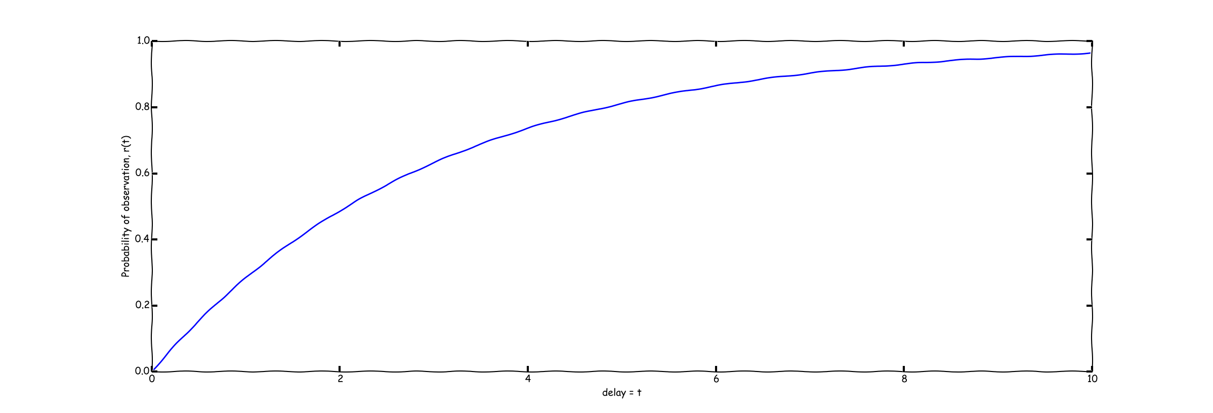
There are a variety of ways of computing $@ r(t) $@ given data, for example the Kaplan-Meier Estimator. Very importantly, one's estimate of $@ r(t) $@ might be probabilistic - this is an issue we'll take up later in this post.
For now, lets assume that $@ r(t) $@ is known.
This means that $@ r(t) $@ is the CDF of the time delay between event and observation, provided of course we know that the observation will eventually occur.
Modelling observations
Let us now consider the question of the probability of an event being observed at a fixed time. We'll first make the observation that:
In contrast, the probability of an event NOT being observed is:
Since we are assuming events and observations are independent of each other, we find that: �
The term here $@ C $@ does not vary with $@ \gamma $@, so we will ignore it. This is safe because, as described earlier, our plan is to numerically integrate the likelihood and find a normalizing constant. If we drop the term $@ C $@ here, then it will be recovered in that calculation.
Does this make sense?
Lets consider two limiting cases as a way to understand whether this result makes intuitive sense. First lets consider the case where $@ T $@ is very large.
In that case, we have:
Ignoring normalizing constants (which don't matter anyway in this analysis), this is proportional to the beta distribution. So in the event that we allow enough time for all events to be observed, we recover the beta distribution for the observation probability $@ \gamma $@.
Lets consider the other limiting case, namely $@ T \rightarrow 0 $@. Since the set of observations is finite, we note that for $@ T < \min_i t_{i,o} $@, no observations have been observed. Thus $@ M = 0 $@ and:
(Note that if there is a finite probability of observing an event after 0 units of time, i.e. if $@ \lim_{t \rightarrow 0} r(t) \neq 0 $@, then this might approach a constant rather than 1.)
What this means is that if we observe the system so early that no events even had time to be observed, then our posterior should not change. I.e., if the experiment has no chance of observing anything, then running the experiment cannot change your beliefs.
So in both of these these limiting cases, this result reproduces exactly what we expect it to.
Implementing it
Now lets consider a data set. We have a sequence of event times as well as observation times:
event_times = array([2.5, 3.7, ... ])
observation_times = array([ 3.6, 5.8, ...])
N = len(event_times)
M = len(observation_times)
assert(M <= N)
We will use this data set to compute a function f(gamma) which is proportional to the likelihood (i.e., it is equal to that function up to a constant factor which does not vary with gamma).
First let us use the fact that $@ x = e^{\log(x)} $@. Then let us note that:
So by implementing this in code, we can gain a numerically stable way of implementing f(gamma). Lets assume we have an implementation of r(t) which is a ufunc (i.e. it can take arrays as entries, and returns arrays of the same shape as output):
def f(gamma):
    x = np.outer(r(T-event_times[M+1:N]), gamma)
    log_likelihood = M*log(gamma) + sum(log(1-x), axis=0)
    return exp(log_likelihood)
The outer product step is probably worth an explanation. Here the variables gamma and event_times are both arrays. So the outer product computes a matrix of the form:
[[ gamma[0] * event_times[0], gamma[0] * event_times[1], gamma[0] * event_times[2], gamma[0] * event_times[3]],
 [ gamma[1] * event_times[0], gamma[1] * event_times[1], gamma[1] * event_times[2], gamma[1] * event_times[3]],
 [ gamma[2] * event_times[0], gamma[2] * event_times[1], gamma[2] * event_times[2], gamma[2] * event_times[3]]
 ]
Now when we compute sum(log(1-x), axis=0) we are first applying the function lambda y: log(1-y) to the elements of this matrix, and then we are computing the sum across the rows of this matrix. As a result, we get another 1-dimensional array containing:
[ log(1-gamma[0]*event_times[0]) + log(1-gamma[0]*event_times[1]) + log(1-gamma[0]*event_times[2]),
  log(1-gamma[1]*event_times[0]) + log(1-gamma[1]*event_times[1]) + log(1-gamma[1]*event_times[2]),
  log(1-gamma[2]*event_times[0]) + log(1-gamma[2]*event_times[1]) + log(1-gamma[2]*event_times[2])
  ]
So by the third line of the function, log_likelihood is an array having the same shape as gamma. The i-th element of this array represents the log likelihood for the specific value gamma[i]. Thus, the function f(gamma) is a genuine ufunc (a function mapping arrays to arrays).
Finally, to compute our actual posterior $@ P(\gamma | t_{e,1}, \ldots, t_{e,N}, t_{o,1}, \ldots, t_{o,N}, T) $@ we do:
gamma = arange(0,1,1/1024.0)

posterior = f(gamma)
posterior /= sum(posterior)
Examples
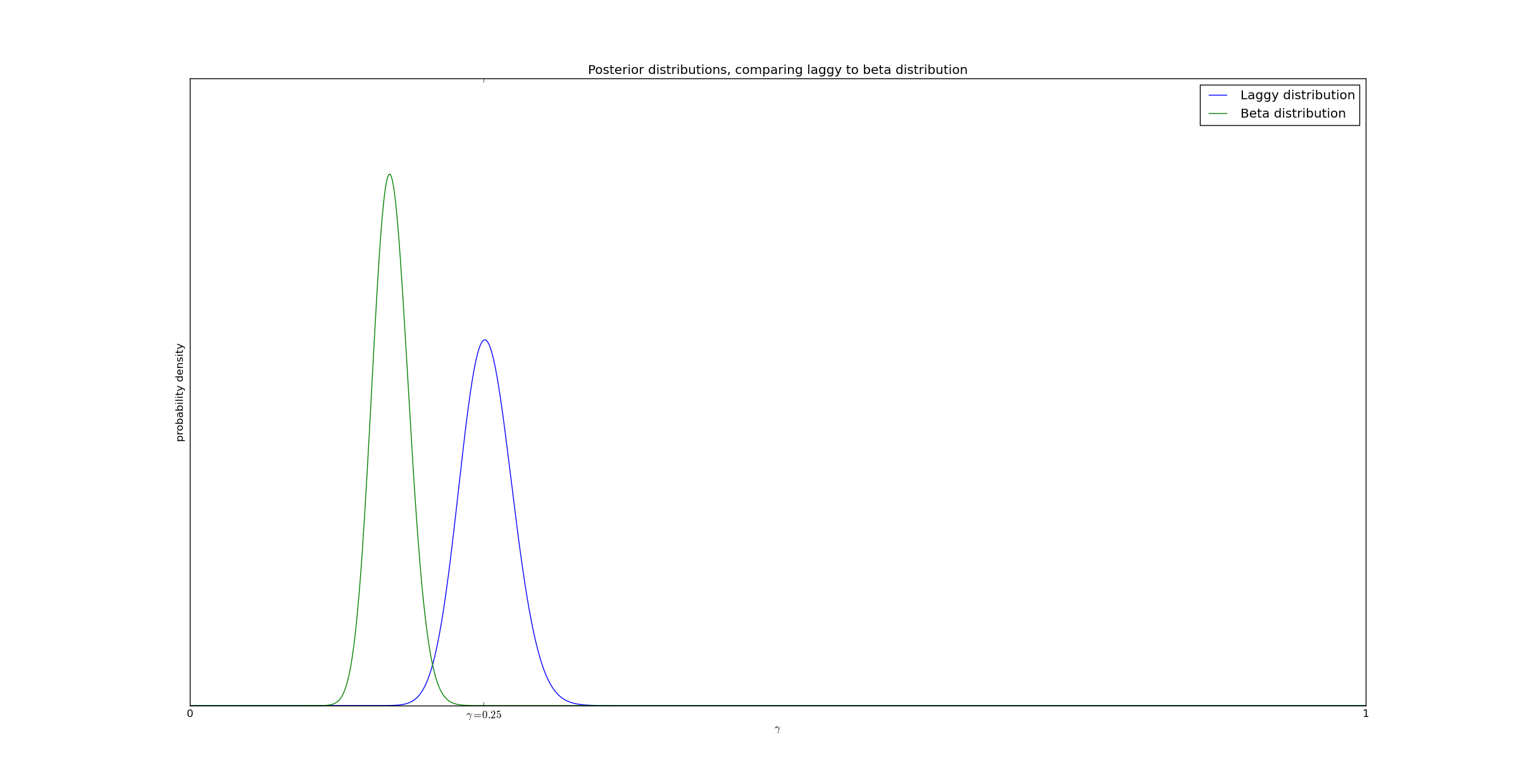
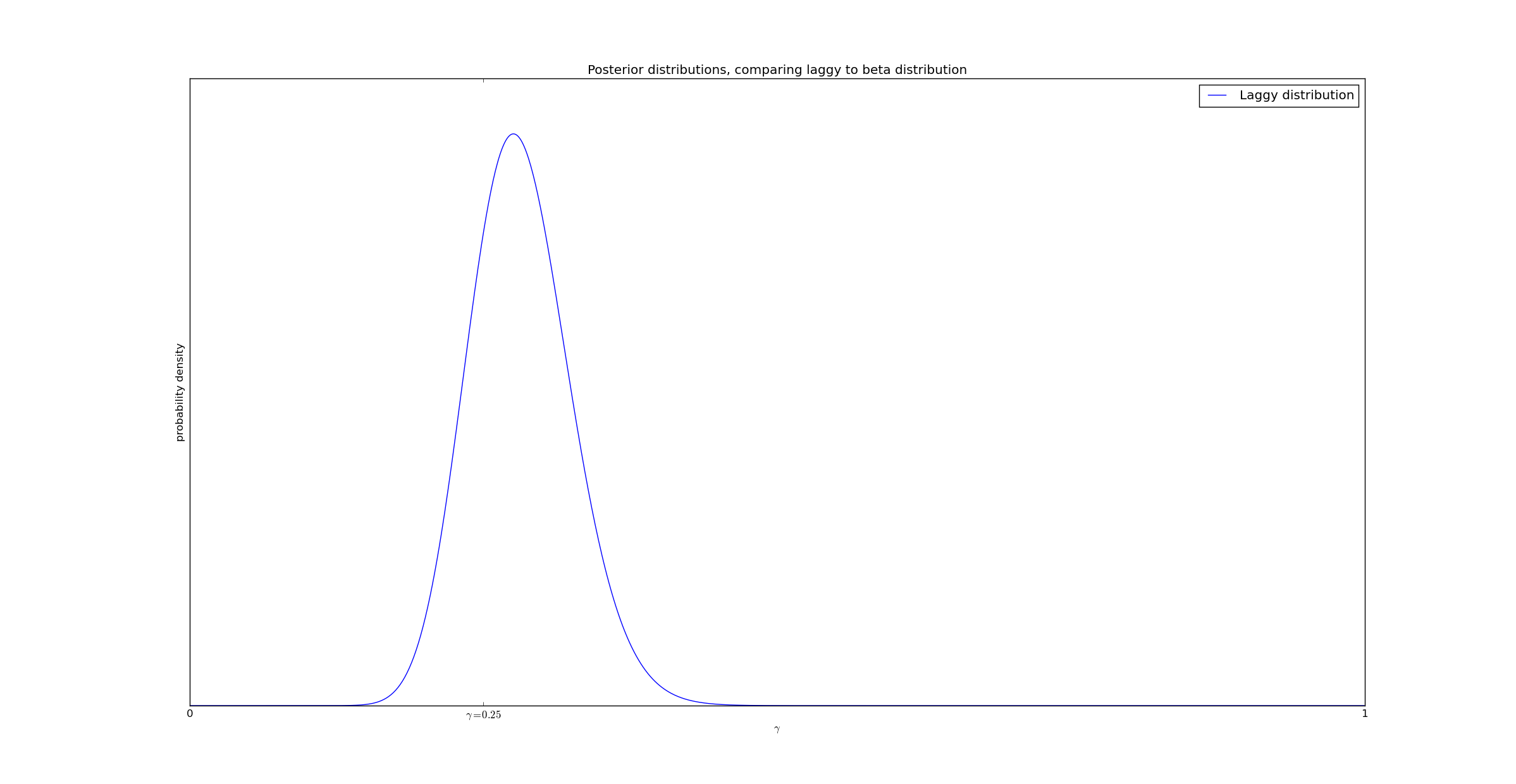
In our first example, I generated data as follows. I had 16 events, with a 25% event detection rate. Events occurred uniformly on the interval \(@ [0,15] $@, and lag was taken to be exponentially distributed with pdf $@ e^{-t/5}\)@. So in this example, there were 600 events and 193 observations which were visible before $@ T = 15 $@.
The posteriors generated by my method, as compared to the classical Beta distribution method, are graphed here:
(Source code for this example is available on github.)
As can be seen from the graph, accounting for delays gives a significantly better result.
If the size of the delay is reduced (from expon(5) to expon(1)), the disparity is significantly reduced, as expected:
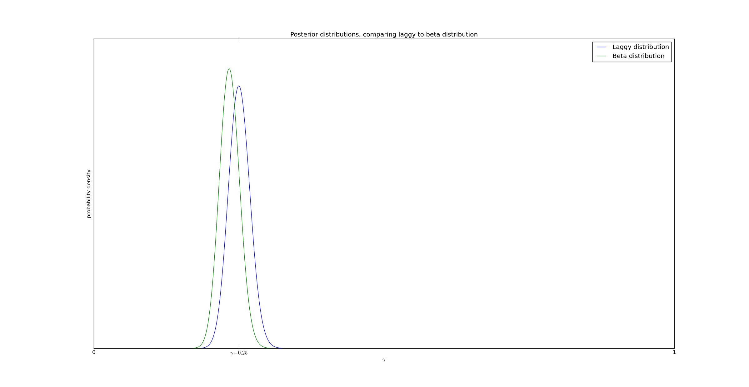
This is to be expected. With a delay of 5 (and a window of [0,15]), approximately 1/3 of the real successes were truncated simply because the test did not finish fast enough to detect them. In contrast, with a delay of 1, only 1/15th of the successes went undetected.
In the third example we will examine what happens when the measurement interval is extremely short. In this example we have 600 data points, but T=2. The mean delay is still 5. This means that most successes will be truncated - we have 600 data points, but only 7 successes before \(@ t = 2\)@.
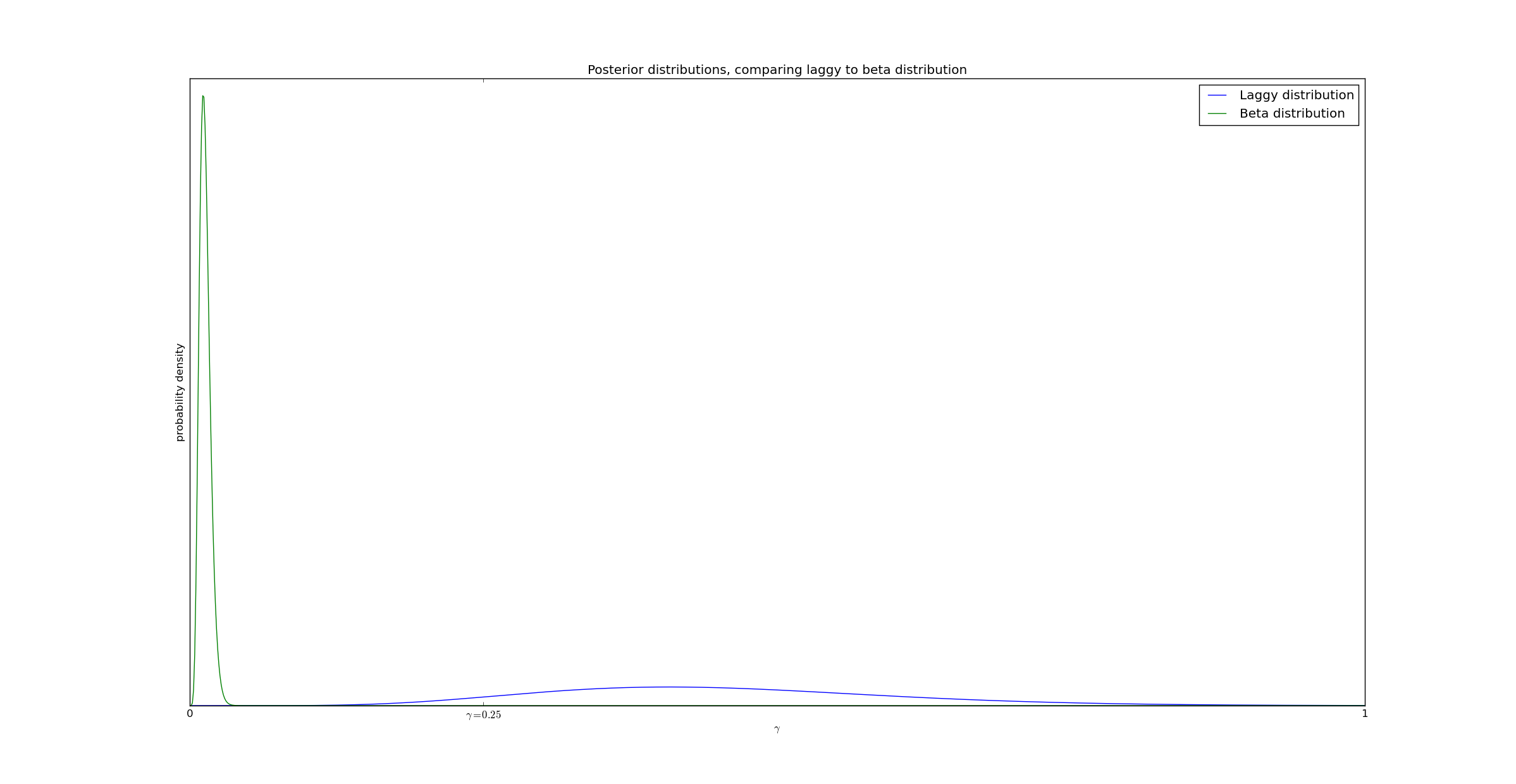
In this example, while the beta distribution gives a highly inaccurate answer, the delayed reaction simply reflects the uncertainty in the estimate.
However, if we have sufficiently many data points we can actually overcome this uncertainty. Consider this case, where we had 6000 events and 39 observations:
If we waited longer than T=2, we would have eventually had 1480 observations. But in spite of 97% of the observations being truncated, we can still measure $@ \gamma $@ with reasonable accuracy!
Conclusion
Delayed reactions can produce significant distortions when computing statistics. However, if the distribution of the delay is known, this effect can be effectively mitigated.
In a later post (I know I keep saying that), I'll illustrate how to mitigate this effect even if $@ r(t) $@ is not well known. I'll give a hint as to how it's done: probability is a monad. In particular, if you have a probability distribution on $@ r(t) $@, you can take that probability distribution and >>= it with what I've done in this post.