Earlier this year I published a blog post about a Baysian decision rule for choosing between two variations, each with a potentially different conversion rate. Later Evan Miller wrote a blog post computing an exact formula for evaluating it, rather than approximating the integral numerically. In this post I'm going to derive an asymptotic expansion of that formula which is valid in the limit of large sample sizes - this is the case when Evan's formula will become computationally difficult to evaluate and prone to numerical error.
The Asymptotic Expansion
The goal is to compute the function:
In terms of Bayesian A/B testing, this function has the definition:
Evan Miller discovered a formula for this, which is somewhat computationally intensive:
This is computationally intensive because a term in the sum must be computed for every data point. However, if we make a scaling assumption, we can derive a much simpler formula. Specifically, let us assume that \(@ a-1=N\phi, b-1=N(1-\phi), c-1=N\psi, d-1=N(1-\psi) $@, with $@ N \rightarrow \infty $@. Provided $@ N $@ is sufficiently large and $@ 0 \leq \phi < \psi \leq 1\)@, we have the approximate formula:
The function $@ B(a,b) $@ is the standard Beta function.
For those unfamiliar with asymptotics, the formula means the following. Suppose we approximate
by
Then the error (expressed as a percentage of the true value) will decay at the rate $@ O(1/N) $@. This can be quantified more precisely, but I don't feel like computing error bounds right now.
If we graph the relative error (namely $@ (\textrm{asymptotic} / \textrm{exact} - 1) $@), we observe the expected behavior:
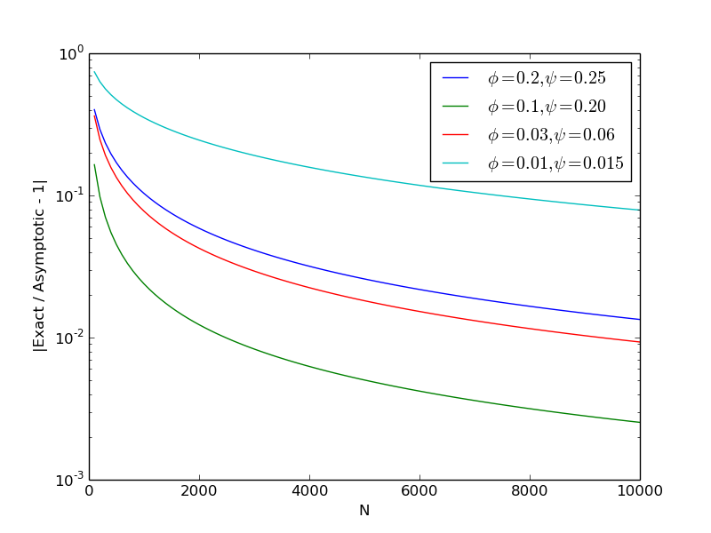
The graph was generated with the following Julia script.
Problems with this method
One flaw with the method described here is that it insists both variants of the A/B test be displayed to the exact same number of users. It is my belief that this assumption can be relaxed. We would instead take the scaling law:
Here $@ \alpha \approx 1 $@, meaning that the two variations no longer need to have the exact same number of users.
Conjecture: The method described here can be made to work with this scaling, and the only result will be minor changes in the formula, of the form $@ \psi \mapsto \alpha \psi $@ and $@ (2-\phi-\psi) \mapsto 1+\alpha-\phi-\alpha\psi $@.
Here comes the math
For any reader unfamiliar with Laplace's method and asymptotic analysis, you can read this free pdf on the topic. The classic (but expensive) textbook is Asymptotics and Special Functions by Olver.
Define $@ C = C(a,b,c,d) \equiv [ B(a,b) B(c,d) ]^{-1} $@ to simplify the notation.
Let us rewrite the integral as the integral of an exponential:
We can then change variables to \(@ u=(x-y)/2 $@ and $@ v = (x+y)/2\)@. Then:
Laplace's Method
At this point we will use Laplace's Method to compute the asymptotics of the integral.
Define the function:
Or equivalently:
Fact: The unique global maxima of $@ \eta(u,v) $@ is achieved at $@ (x,y) = (\phi, \psi) $@. There are no local maxima.
The interesting case is when $@ \phi < \psi $@. This puts the maxima of $@ \eta(x,y) $@ in top left corner, whereas the region being integrated is in the lower right side. This corresponds to the case when $@ P( \textrm{version B is better than Version A}) < 1/2 $@, and we want to determine by how much it is better.
The grunt work
If \(@ \phi < \psi\)@, the maxima of $@ \eta(u,v) $@ is in the top left side of the unit square, while the region of integration is the lower right side. This means that for the inner integral, the maxima of $@ \eta(x,y) $@ is achieved at the left endpoint $@ u=0 $@. Applying Laplace's method, we find:
A simple computation shows that:
And also:
Substituting this in, we have:
We can now plug this formula into the definition of \(@ g( N\phi, N(1-\phi), N\psi, N(1-\psi))\)@:
The reader will observe that this integral is the definition of the Beta function.
This is what we wanted to show.
In principle higher order terms can also be computed, but that seems unnecessary at this point. I believe the approach in section 3 of Asymptotic Inversion of the Incopmlete Beta Function may also be useful.