Consider a data set, a sequence of point \(@ (x_1, y_1), (x_2, y_2), \ldots, (x_k, y_k)\)@. We are interested in discovering the relationship between x and y. Linear regression, at it's simplest, assumes a relationship between x and y of the form \(@ y = \alpha x + \beta + e\)@. Here, the variable $@ e $@ is a noise term - it's a random variable that is independent of $@ x $@, and varies from observation to observation. This assumed relationship is called the model.

(In the case where x is a vector, the relationship is assumed to take the form \(@ y = \alpha \cdot x + \beta + e\)@. But we won't get into that in this post.)

The problem of linear regression is then to estimate $@ \alpha, \beta $@ and possibly $@ e $@.

In this blog post, I'll approach this problem from a Bayesian point of view. Ordinary linear regression (as taught in introductory statistics textbooks) offers a recipe which works great under a few circumstances, but has a variety of weaknesses. These weaknesses include an extreme sensitivity to outliers, an inability to incorporate priors, and little ability to quantify uncertainty.

Bayesian linear regression (BLR) offers a very different way to think about things. Combined with some computation (and note - computationally it's a LOT harder than ordinary least squares), one can easily formulate and solve a very flexible model that addresses most of the problems with ordinary least squares.

The simplest version

To begin with, let's assume we have a one-dimensional dataset $@ (x_1, y_1), \ldots, (x_k, y_k) $@. The goal is to predict $@ y_i $@ as a function of $@ x_i $@. Our model describing $@ y_i $@ is

where $@ \alpha $@ and $@ \beta $@ are unknown parameters, and $@ e $@ is the statistical noise. In the Bayesian approach, $@ \alpha $@ and $@ \beta $@ are unknown, and all we can do is form an opinion (compute a posterior) about what they might be.

To start off, we'll assume that our observations are independent and identically distributed. This means that for every $@ i $@, we have that:

where each $@ e_i $@ is a random variable. Let's assume that $@ e_i $@ is an absolutely continuous random variable, which means that it has a probability density function given by $@ E(t) $@.

Our goal will be to compute a posterior on $@ (\alpha, \beta) $@, i.e. a probability distribution $@ p(\alpha,\beta) $@ that represents our degree of belief that any particular $@ (\alpha,\beta) $@ is the "correct" one.

At this point it's useful to compare and contrast standard linear regression to the bayesian variety.

In standard linear regression, your goal is to find a single estimator $@ \hat{\alpha} $@. Then for any unknown $@ x $@, you get a point predictor $@ y_{approx} = \hat{\alpha} \cdot x $@.

In bayesian linear regression, you get a probability distribution representing your degree of belief as to how likely $@ \alpha $@ is. Then for any unknown $@ x $@, you get a probability distribution on $@ y $@ representing how likely $@ y $@ is. Specifically:

Computing Posteriors with PyMC

To compute the posteriors on $@ (\alpha, \beta) $@ in Python, we first import the PyMC library:

import pymc

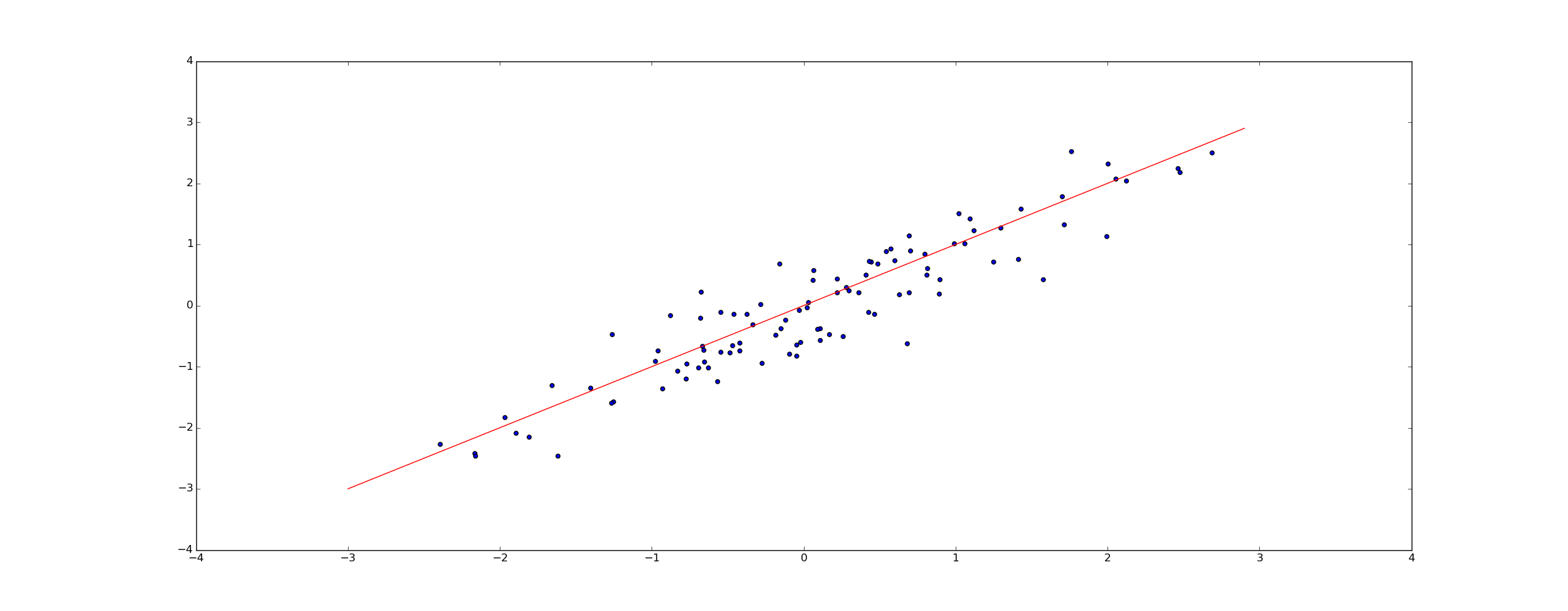
We then generate our data set (since this is a simulation), or otherwise load it from an original data source:

from scipy.stats import norm

k = 100 #number of data points
x_data = norm(0,1).rvs(k)
y_data = x_data + norm(0,0.35).rvs(k) + 0.5

We then define priors on $@ (\alpha, \beta) $@. In this case, we'll choose uniform priors on [-5,5]:

alpha = pymc.Uniform('alpha', lower=-5, upper=5)
beta = pymc.Uniform('beta', lower=-5, upper=5)

Finally, we define our observations.

x = pymc.Normal('x', mu=0,tau=1,value=x_data, observed=True)

@pymc.deterministic(plot=False)
def linear_regress(x=x, alpha=alpha, beta=beta):
    return x*alpha+beta

y = pymc.Normal('output', mu=linear_regress, value=y_data, observed=True)

Note that for the values x and y, we've told PyMC that these values are known quantities that we obtained from observation. Then we run to some Markov Chain Monte Carlo:

model = pymc.Model([x, y, alpha, beta])
mcmc = pymc.MCMC(model)
mcmc.sample(iter=100000, burn=10000, thin=10)

We can then draw samples from the posteriors on alpha and beta:

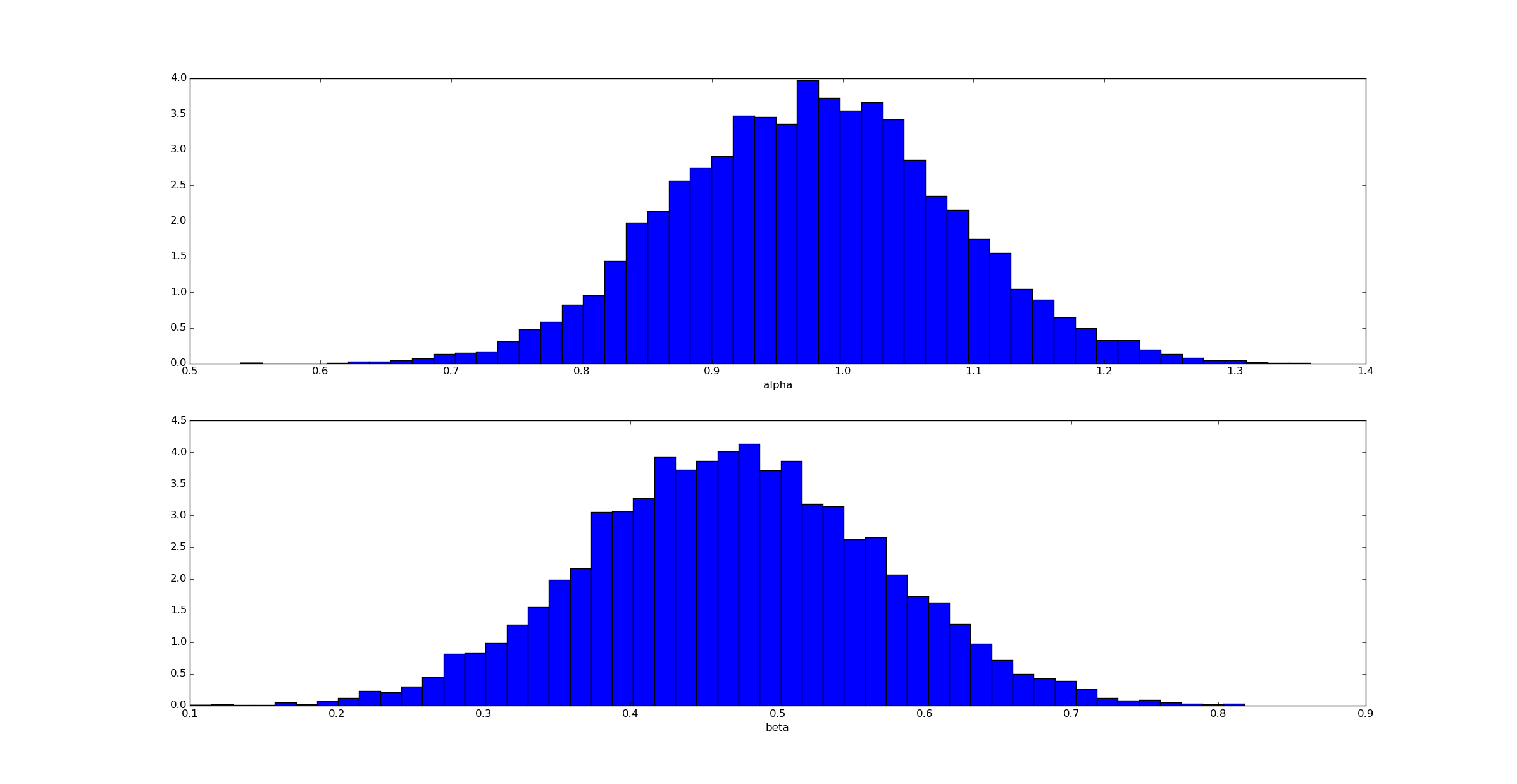
Unsurprisingly (given how we generated the data) the posterior for $@ \alpha $@ is clustered near $@ \alpha=1 $@ and for $@ \beta $@ near $@ \beta=0.5 $@.

We can then draw a sample of regression lines:

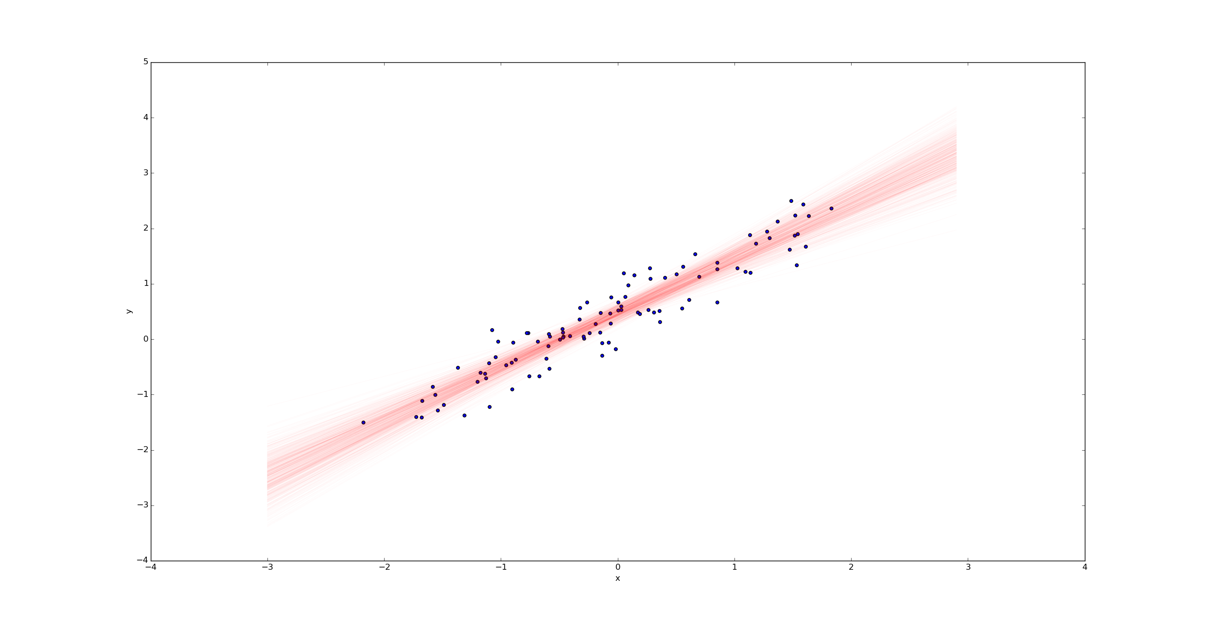
Unlike in the ordinary linear regression case, we don't get a single regression line - we get a probability distribution on the space of all such lines. The width of this posterior represents the uncertainty in our estimate.

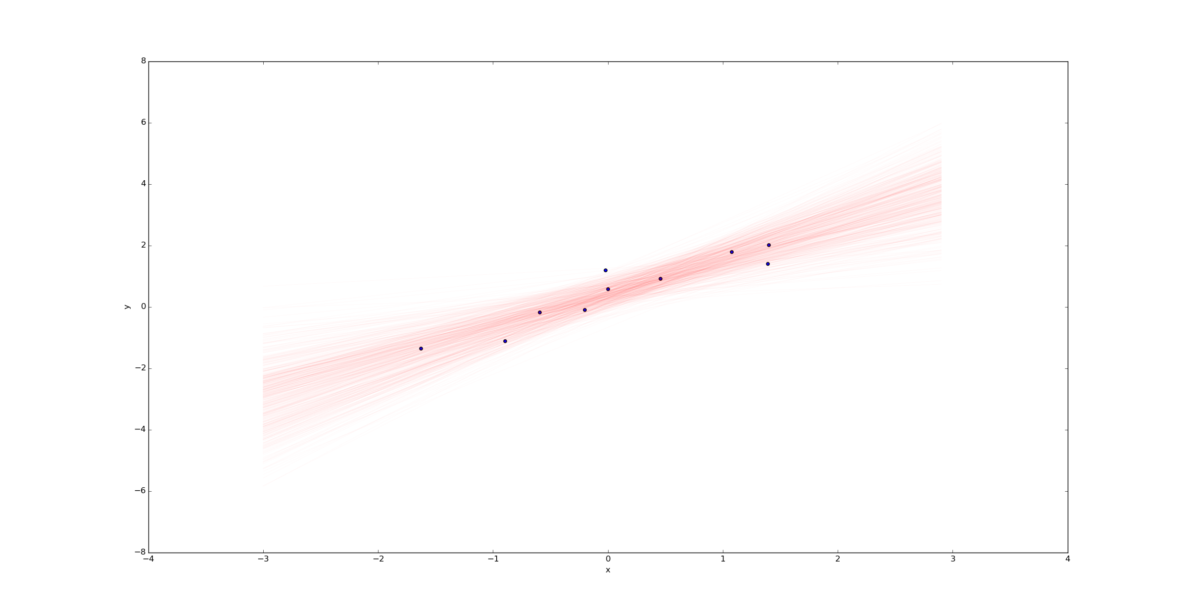
Imagine we were to change the variable k to k=10 in the beginning of the python script above. Then we would have only 10 samples (rather than 100) and we'd expect much more uncertainty. Plotting a sample of regression lines reveals this uncertainty:

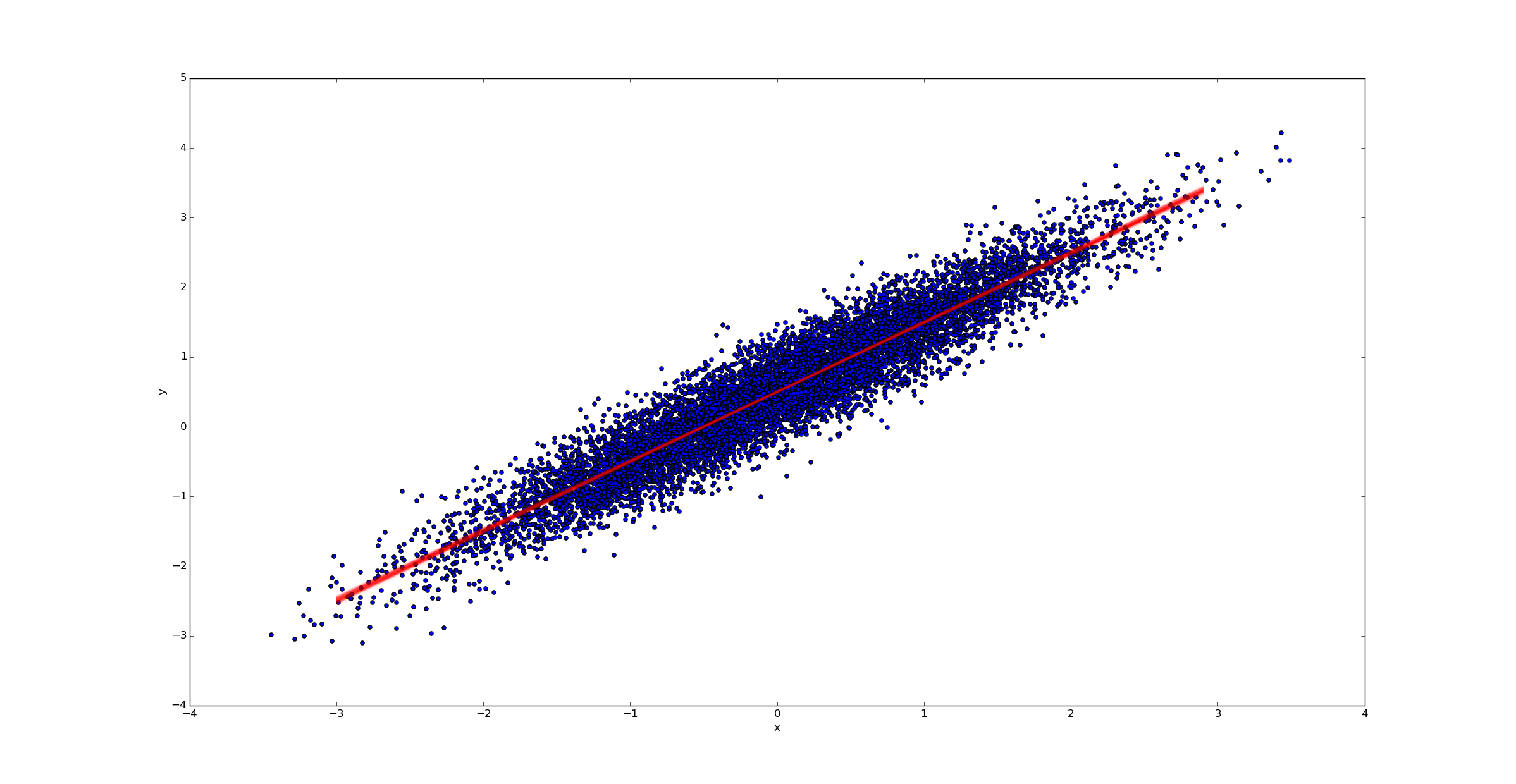
In contrast, if we had far more samples (say k=10000), we would have far less uncertainty in the best fit line:

Handling outliers

In many classical statistics textbooks, the concept of an "outlier" is introduced. Textbooks often treat outliers as data points which need to be specially treated - often ignored - because they don't fit the model and can heavily skew results.

Consider the following example. 50 data points were generated. In the left graph, the y-values were chosen according to the rule $@ y = 1.0 x + 0.5 + e $@ where $@ e $@ is drawn from a normal distribution. In the right graph, the y-values were chosen according to the same rule, but with $@ e $@ drawn from a Cauchy distribution. I then did ordinary least squares regression to find the best fit line.

The red line in the graph is the best fit line, while the green line is the true relation.

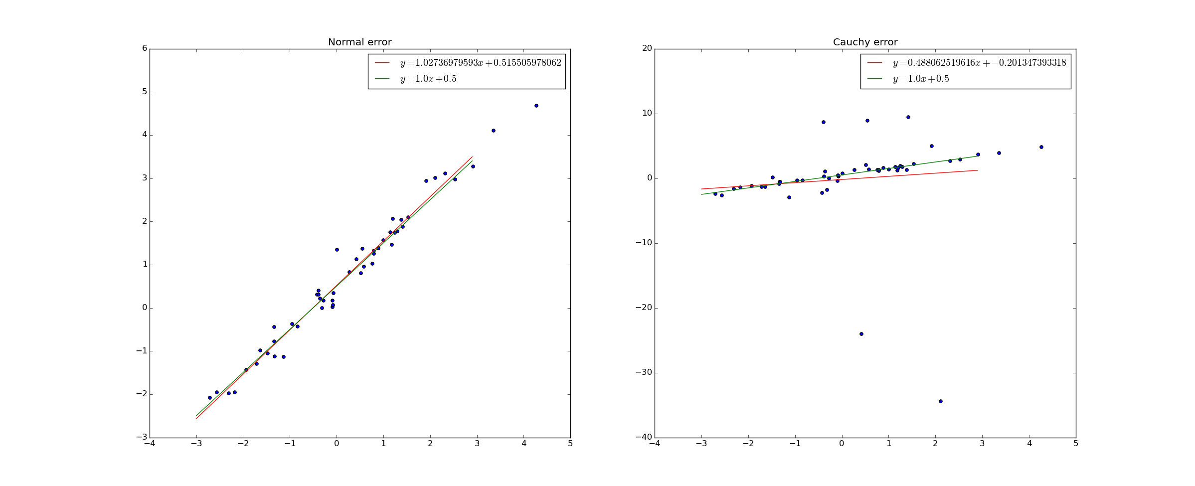
The Cauchy distribution is actually pretty pathological - it's variance is infinite. The result of this is that "outliers" are not actually uncommon at all - extremely large deviations from the mean are perfectly normal.

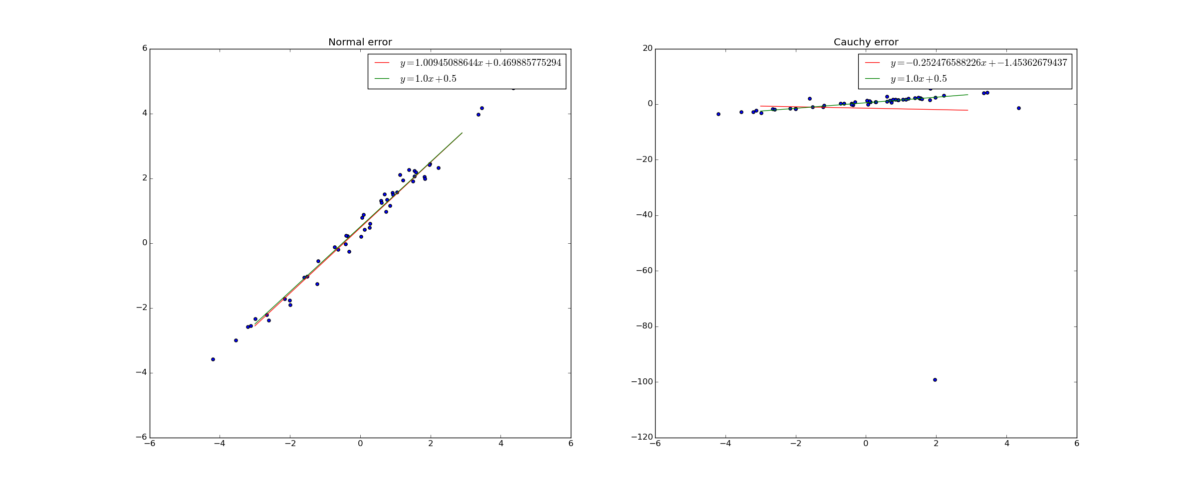
With a normal distribution, the probability of seeing a data point at \(@ y=-20\)@ or $@ -30 $@ (as described in the figure) is very small, particularly if the line is sloping upward. As a result, the fact that such a data point did occur is very strong evidence in favor of the line having a much smaller upward slope - even though only a few points slope this way.

In fact, a sufficiently large singleton "outlier" can actually shift the slope of the best fit line from positive to negative:

However, if we use Bayesian linear regression and simply change the distribution on the error in Y to a cauchy distribution, Bayesian linear regression adapts perfectly:

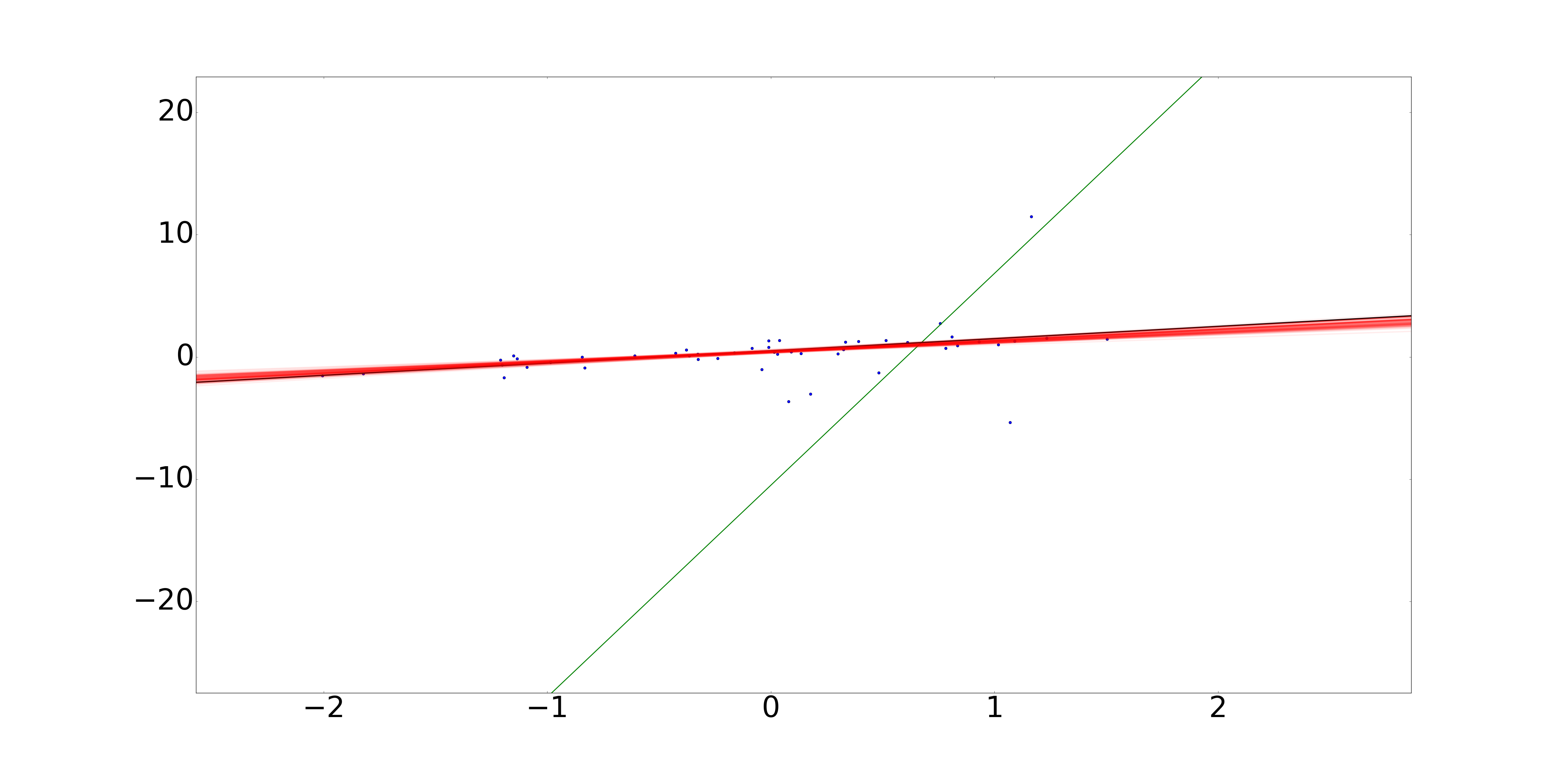
In this picture, we have 50 data points with Cauchy-distributed errors. The black line represents the true line used to generate the data. The green line represents the best possible least squares fit, which is driven primarily by the data point at (1, 10). The red lines represent samples drawn from the Bayesian posterior on $@ (\alpha, \beta) $@.

In code, all I did to make this fix was:

-y = pymc.Normal('output', mu=linear_regress, value=y_data, observed=True)
+y = pymc.Cauchy('output', alpha=linear_regress, beta=0.35, value=y_data, observed=True)

This fairly simple fix helps the model to recover.

Where does ordinary least squares come from? Maximal likelihood.

Rather than simply setting up a somewhat overcomplicated model in PyMC, one can also set up the MCMC directly. Supposing we have a data set \(@D = \{ (x_i, y_i) \}\)@. Then:

If the samples are i.i.d, we can write this as:

Because we assumed the error term has a PDF and is additive, we can simplify this to:

Given this formulation, we have now expressed the posterior as being proportional to a known function. This allows us to run any reasonable Markov Chain Monte Carlo algorithm directly and draw samples from the posterior.

Suppose we now choose a very particular distribution - suppose we take $@ E(t) = C e^{-t^2/2} $@. Further, suppose take an uninformative (and improper) prior, namely $@ \textrm{prior}(\alpha, \beta) = 1 $@ - this means we have literally no information on $@ \alpha $@ before we start. In this case:

If we attempt to maximize this quantity (or it's log) in order to find the point of maximum likelihood, we obtain the problem:

Here the argmax is computed over $@ (\alpha, \beta) $@. This is precisely the problem of minimizing the squared error. So an uninformative prior combined with a Gaussian error term allows Bayesian Linear Regression to revert to ordinary least squares.

One very important fact is that because OLS computes the peak of BLR, one can think of OLS as being a cheap approximation to BLR.

Easier modeling, uncertainty representation

Bayesian Linear Regression is an important alternative to ordinary least squares. Even if you don't use it often due to it's computationally intensive nature, it's worth thinking about as a conceptual aid.

Whenever I think of breaking out least squares, I work through the steps of BLR in my head.

1. Are my errors normally distributed or close to it?
2. Do I have enough data so that my posterior will be narrow?

In the event that these assumptions are true, it's reasonably safe to use OLS as a computationally cheap approximation to BLR.

Sometimes the approximations simply aren't true. For example, a stock trading strategy I ran for a while had a very strong requirement of non-normal errors. Once I put the non-normal errors in, and quantified uncertainty (i.e. error in the slope and intercept of the line), my strategy went from losing $1500/month to gaining $500/month.

For this reason I encourage thinking of regression in Bayesian terms. I've adopted this in my thinking and I find the benefits vastly exceed the costs.