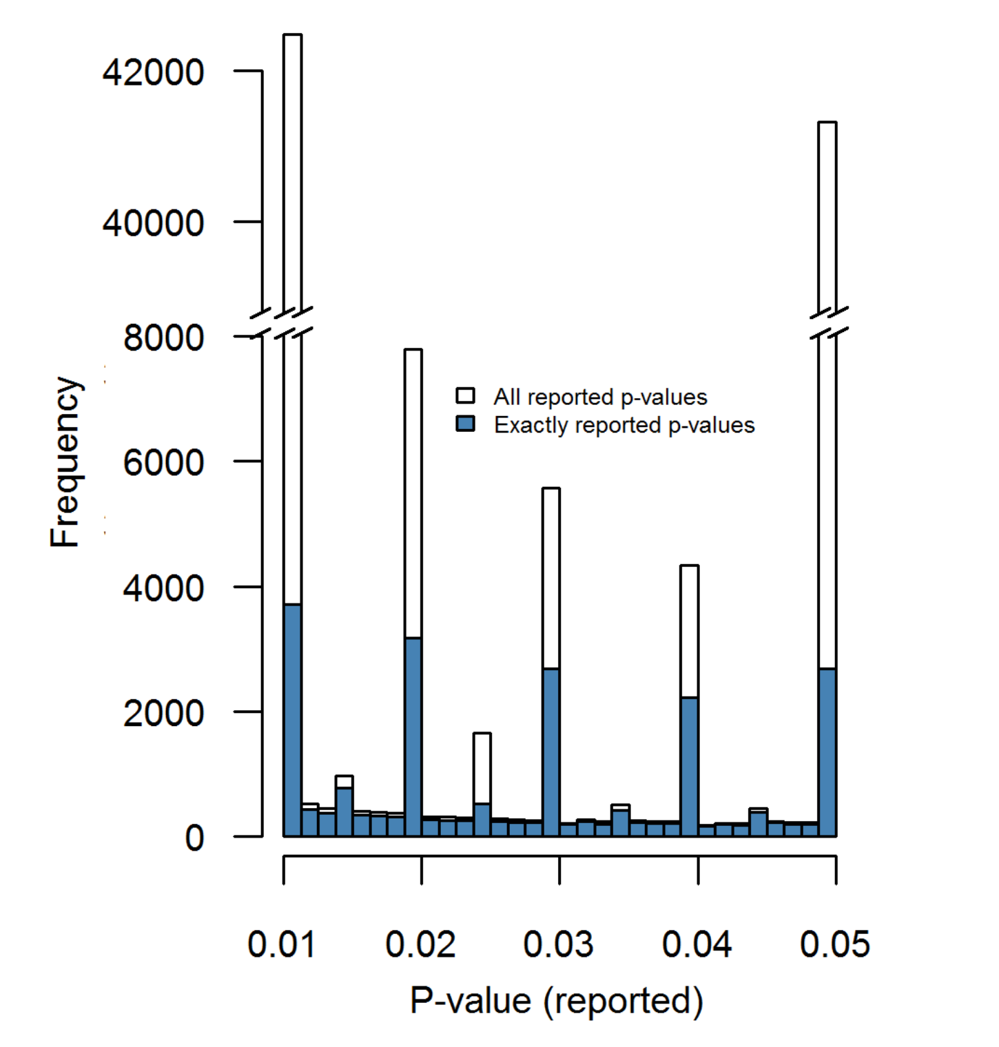
A lot of suspicious behavior can be detected simply by looking at a histogram. Here's a nice example. There's a paper Distributions of p-values smaller than .05 in Psychology: What is going on? which attempts to characterize the level of data manipulation performed in academic psychology. Now under normal circumstances, one would expect a nice smooth distribution of p-values resulting from honest statistical analysis.
What actually shows up when they measure it is something else entirely:
Another example happened to me when I was doing credit underwriting. A front-line team came to me with concerns that some of our customers might not be genuine, and in fact some of them might be committing fraud! Curious, I started digging into the data and made a histogram to get an idea of spending per customer. The graph looked something like this:
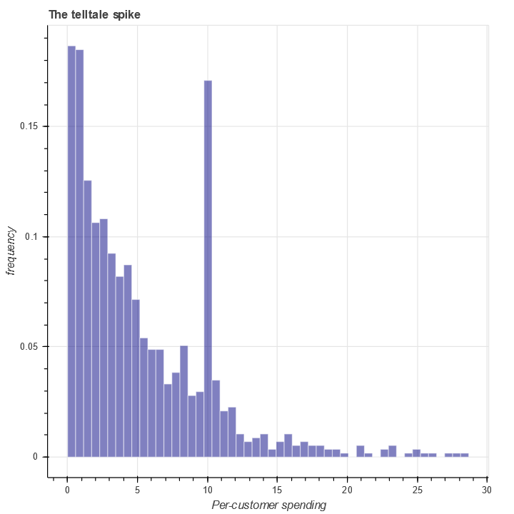
The value x=10 corresponded to the credit limit we were giving out to many of our customers. For some reason, a certain cohort of users were spending as much as possible on the credit lines we gave them. Further investigation determined that most of those customers were not repaying the money we lent them.
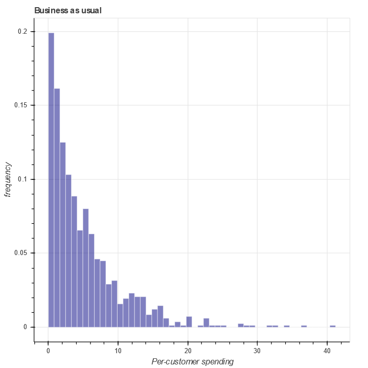
In contrast, under normal circumstances, a graph of the same quantity would typically kook like this:
A third example - with graphs very similar to the previous example - happened to me when debugging some DB performance issues. We had a database in US-East which was replicated to US-West. Read performance in US-West was weirdly slow, and when we made a histogram of request times, it turned out that the slowness was driven primarily by a spike at around 90ms. Coincidentally, 90ms was the ping time between our US-East and US-West servers. It turned out that a misconfiguration resulted in the US-West servers occasionally querying the US-East read replica instead of the US-West one, adding 90ms to the latency.
A fourth example comes from the paper Under Pressure? Performance Evaluation of Police Officers as an Incentive to Cheat: Evidence from Drug Crimes in Russia which discovers odd spikes in the amount of drugs found in police searches.
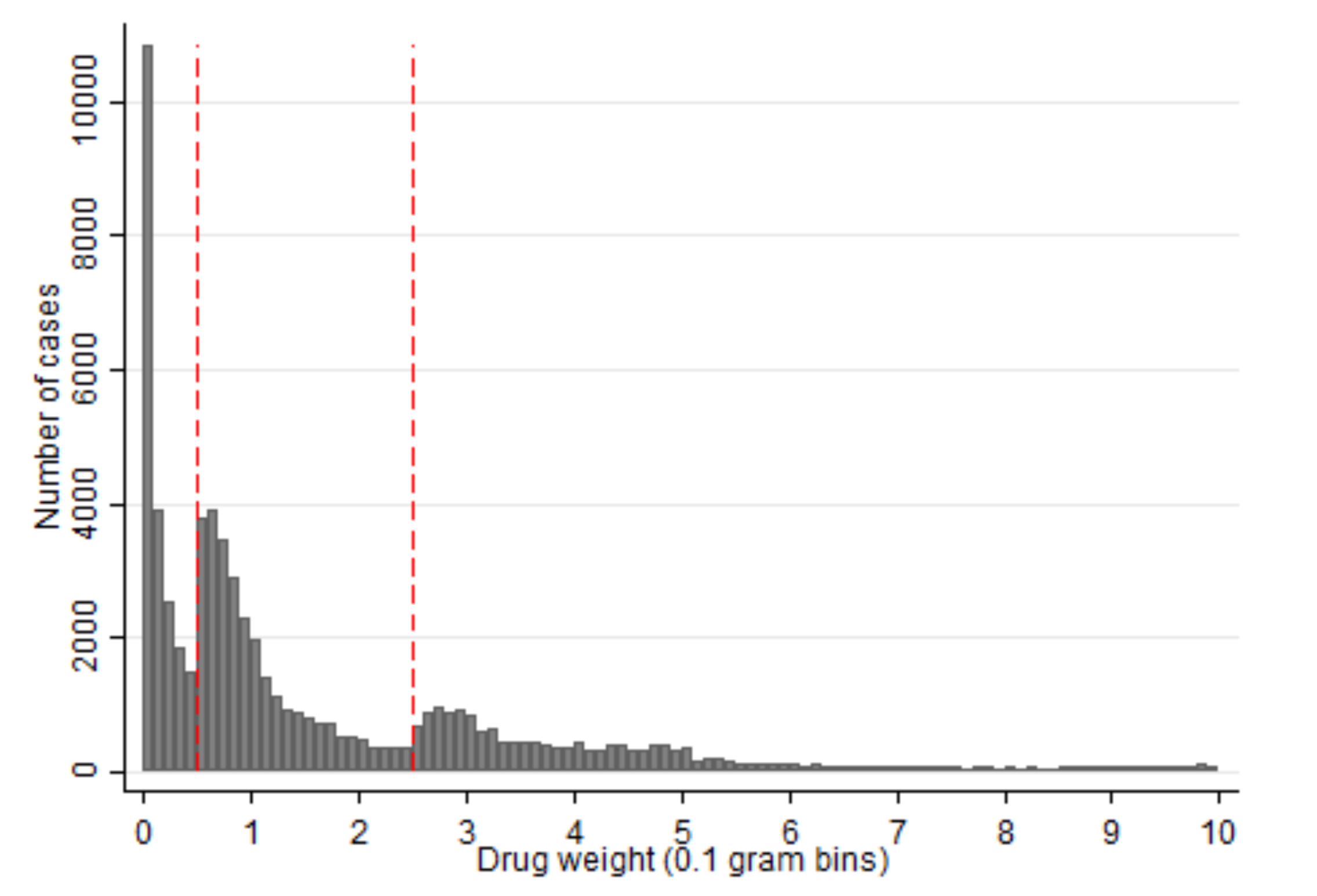
It sure is very strange that so many criminals all choose to carry the exact amount of heroin needed to trigger harsher sentencing thresholds, and never a few grams less.
In short, many histograms should be relatively smooth and decreasing. When such histograms display a spike, that spike is a warning sign that something is wrong and we should give it further attention.
In all the cases above, I made these histograms as part of a post-hoc analysis. Once the existence of a problem was suspected, further evidence was gathered and the spike in the histogram was one piece of evidence. I've always been interested in the question - can we instead automatically scan histograms for spikes like the above and alert humans to a possible problem when they arise?
This blog post answers the question in the affirmative, at least theoretically.
Mathematically modeling a single test
To model this problem in the frequentist hypothesis testing framework, let us assume we have a continuous probability distributions \(f\) which is supported on \([0,\infty)\). As our null hypothesis - i.e. nothing unusual to report - we'll assume this distribution is absolutely continuous with respect to Lebesgue measure and that it has pdf \(f(x) dx\) which is monotonically decreasing, i.e. \(f(y) \leq f(x)\) for \(y \geq x\) (almost everywhere).
In contrast, for the alternative hypothesis - something worth flagging as potentially bad - I'll assume that the distribution is a mixture distribution with pdf \((1-\beta) f(x) + \beta s(x) dx\). Here \(s(x)\) is monotonically increasing, or more typically \(s(x) = \delta(x-x_0)\).
Observation: Consider a probability distribution \(f(x)\) that is monotonically decreasing. Then the cumulative distribution function \(F(x)=\int_0^x f(t) dt\) is concave. This can be proven by noting that it's derivative, \(F'(x) = f(x)\) is monotonically decreasing.
Our hypothesis test for distinguishing between the null and alternative hypothesis will be based on concavity. Specifically, if there are spikes in a histogram of the pdf of a distribution, then it's CDF may cease to be concave at the point of the spike. Here's an illustration. First, consider the empirical CDF of a distribution which is monotonically decreasing:
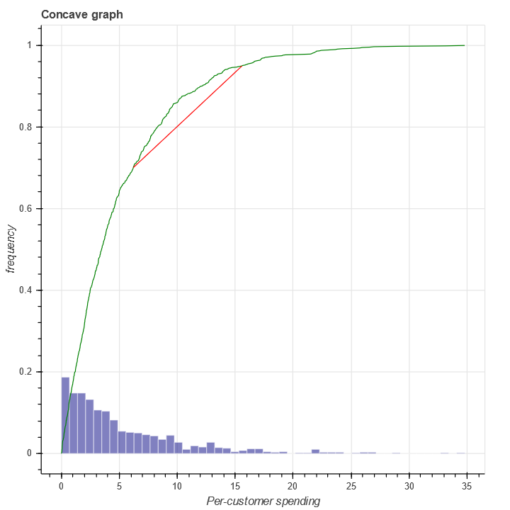
This graph is clearly concave. The red line illustrates a chord which must, by concavity, remain below the actual curve.
In contrast, a pdf with a spike in it will fail to be concave near the spike. Here's an illustration:
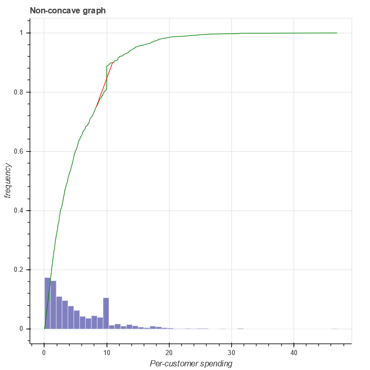
At \(x=10\) the chord (the red line) is above the graph of the CDF (the green line).
In mathematical terms, concavity of the true CDF can be expressed as the relation:
or equivalently:
Since we do not know \(F(x)\) exactly, we of course cannot measure this directly. But given a sample, we can construct the empirical CDF which is nearly as good:
Using the empirical CDF and the definition of concavity suggests a test statistic which we can use:
Our goal is to show that if this test statistic is sufficiently negative, then a spike must exist.
When \(q\) becomes negative, this shows that \(F_n(x)\) is non-concave. However, the empirical distribution function is by definition non-concave, as can be seen clearly when we zoom in:
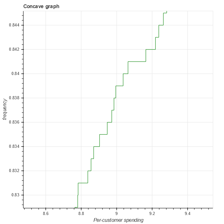
Mathematically we can also see this simply by noting that \(1_{x \geq x_i}\) is not concave. However, this non-concavity has order of magnitude \(O(n^{-1})\), so to deal with this we can simply demand that \(q < -1/n\).
There is a larger problem caused - potentially - by deviation between the empirical distribution \(F_n(x)\) and the true, continuous and concave cdf \(F(x)\). This however can also be controlled and will be controlled in the next section.
Controlling false positives
To control false positives, there is a useful mathematical tool we can use to control this - the DKW inequality (abbreviating Dvoretzky–Kiefer–Wolfowitz). This is a stronger version of the Glivenko-Cantelli Theorem, but which provides uniform convergence over the range of the cdf.
We use it as follows.
Recall that \(q\) is defind as a minima of \(\left[ F_n(x+\alpha(y-x)) - (1-\alpha)F_n(x) - \alpha F_n(y)\right]\). Let us choose \((x,y,\alpha)\) now to be the value at which that minima is achieved. Note that this requires that \(x < y\) are two points in the domain of \(F(x)\) and \(\alpha \in [0,1]\). Let us also define \(z=x + \alpha(y-x)\) in order to simplify the calculation.
Now lets do some arithmetic, starting from the definition of concavity of the CDF:
(This line follows since \(\left[ F_n(x+\alpha(y-x)) - (1-\alpha)F_n(x) - \alpha F_n(y)\right] = q\) due to our choice of \((x,y,\alpha)\) above.)
The DKW inequality tells us that for any \(\epsilon > 0\),
Substituting this into the above, we can therefore say that with probability \(e^{-2n\epsilon^2}\),
If \(q + 2\epsilon < 0\), this lets us reject the null hypothesis that \(F(x)\) is concave, or equivalently, that \(f(x)\) is monotonically decreasing. Conversely, given a value of \(q\), we can invert to gain a p-value. We summarize this as a theorem:
Theorem 1: Assume the null hypothesis of concavity is true. Let \(q\) be defined as above. Then if \(q < 0\), we can reject the null hypothesis (that \(f(x)\) is decreasing monotonically) with p-value \(p=e^{-n q^2/2}\).
This convergence is exponential but at a slow rate. Much like a Kolmogorov-Smirnov, the statistical power is relatively low compared to parametric tests (such as Anderson-Darling) that are not based on the DKW inequality.
Controlling true positives
Let us now examine the true positive rate and attempt to compute statistical power. As a simple alternative hypothesis, let us take a mixture model:
Here \(f(x)\) is monotone decreasing and \(\delta(x-x_0)\) is the point mass at \(x_0\). Let us attempt to compute
Let \(x=x_0-\epsilon\), \(y=x_0+\epsilon^2\) and \(\alpha=\frac{1-\epsilon}{1+\epsilon}\). Then:
Now substituting this in, we discover:
Letting \(\bar{F}(x) = \int_0^x f(x) dx\), we observe that \(F(x) = (1-\beta)\bar{F}(x) + 1_{x \geq x_0}\). Since \(f(x)\) is absolutely continuous, \(\bar{F}(x)\) is of course a continuous function.
Let us now take the limit as \(\epsilon \rightarrow 0\):
This implies that
since the minima is of course smaller than any limit.
By the same argument as in the previous section - using the DKQ inequality to relate \(F(x)\) to \(F_n(x)\) - we can therefore conclude that:
with probability \(1-e^{-2n\epsilon^2}\).
Distinguishing the null and alternative hypothesis
We can combine these results into a hypothesis test which is capable of distinguishing between the null and alternative hypothesis with any desired statistical power.
Theorem 2: Let \(p\) be a specified p-value threshold and let \(r\) be a desired statistical power. Let us reject the null hypothesis whenever
Suppose now that
Then with probability at least \(r\), we will reject the null hypothesis.
Example numbers and slow convergence
Due to the slowness of the convergence implied by the DKW inequality, we unfortunately need fairly large \(n\) (or large \(\beta\)) for this test to be useful.
| n | \(\beta\) |
|---|---|
| 1000 | 0.155 |
| 2000 | 0.109 |
| 5000 | 0.0692 |
| 10000 | 0.0490 |
| 25000 | 0.0310 |
| 100000 | 0.0155 |
Thus, this method is really only suitable for detecting either large anomalies or in situations with large sample sizes.
Somewhat importantly, this method is not particularly sensitive to the p-value cutoff. For example, with a 1% cutoff rather than a 5%, we can detect spikes of size \(\beta=0.055\) at \(n=10000\).
This makes the method reasonably suitable for surveillance purposes. By setting the p-value cutoff reasonably low (e.g. 1% or 0.1%), we sacrifice very little measurement power on a per-test basis. This allows us to run many versions of this test in parallel and then use either the Sidak correction to control the group-wise false positive rate or Benjamini-Hochburg to control the false discovery rate.
Conclusion
At the moment this test is not all I was hoping for. It's quite versatile, in the sense of being fully nonparametric and assuming little beyond the underlying distribution being monotone decreasing. But while theoretically the convergence is what one would expect, in practice the constants involved are large. I can only detect spikes in histograms after they've become significantly larger than I'd otherwise like.
However, it's still certainly better than nothing. This method would have worked in several of the practical examples I described at the beginning and would have flagged issues earlier than than I detected them via manual processes. I do believe this method is worth adding to suites of automated anomaly detection. But if anyone can think of ways to improve this method, I'd love to hear about them.
I've searched, but haven't found a lot of papers on this. One of the closest related ones is Multiscale Testing of Qualitative Hypotheses.