Frequently in data science, we have a relationship between X and y where (probabilistically) y increases as X does. The relationship is often not linear, but rather reflects something more complex. Here's an example of a relationship like this:
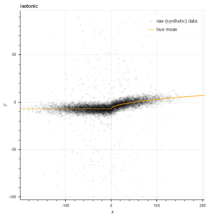
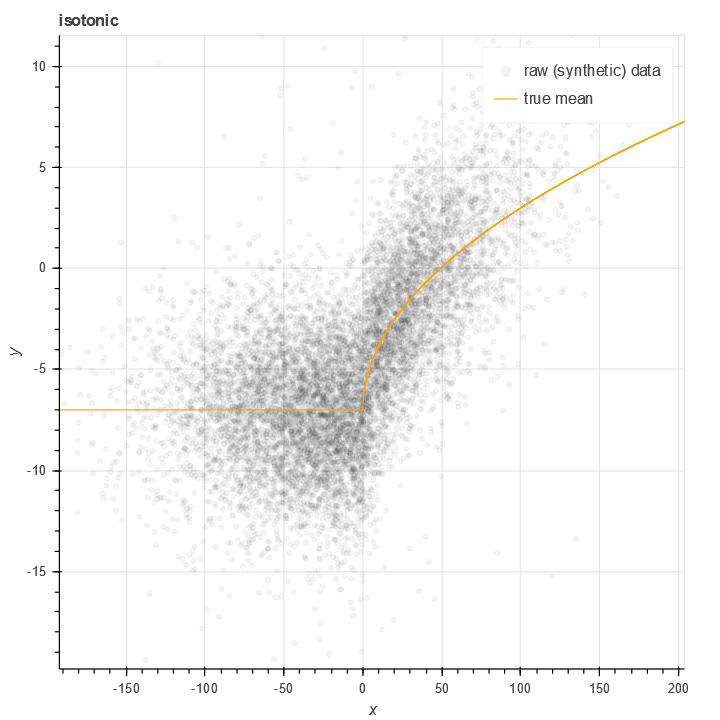
In this plot of synthetic we have a non-linear but increasing relationship between X and Y. The orange line represents the true mean of this data. Note the large amount of noise present.
There is a classical algorithm for solving this problem nonparametrically, specifically Isotonic regression. This simple algorithm is also implemented in sklearn.isotonic. The classic algorithm is based on a piecewise constant approximation - with nodes at every data point - as well as minimizing (possibly weighted) l^2 error.
The standard isotonic package works reasonably well, but there are a number of things I don't like about it. My data is often noisy with fatter than normal tails, which means that minimizing l^2 error overweights outliers. Additionally, at the endpoints, sklearn's isotonic regression tends to be quite noisy.
The curves output by sklearn's isotonic model are piecewise constant with a large number of discontinuities (O(N) of them).
The size of the isotonic model can be very large - O(N), in fact (with N the size of the training data). This is because in principle, the classical version isotonic regression allows every single value of x to be a node.
The isotonic package I've written provides some modest improvements on this. It uses piecewise linear curves with a bounded (controllable) number of nodes - in this example, 30:
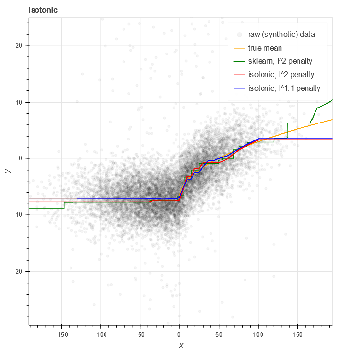
It also allows for non-l^2 penalties in order to handle noise better.
Isotonic regression for binary data
Another issue facing the standard isotonic regression model is binary data - where y in [0,1]. Using RMS on binary data sometimes works (when there's lots of data and it's mean is far from 0 and 1), but it's far from optimal.
For this reason I wrote a class isotonic.BinomialIsotonicRegression which handles isotonic regression for the case of a binomial loss function.
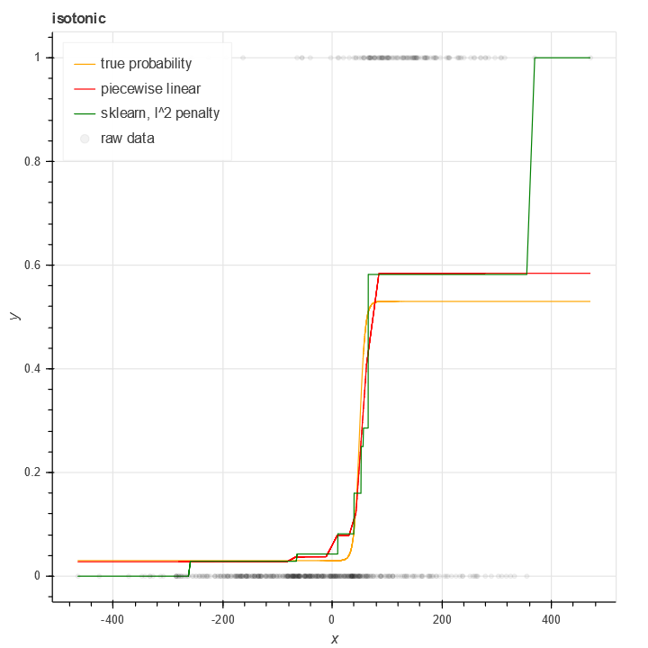
As is apparent from the figure, this generates more plausible results for binary isotonic regression (in a case with relatively few samples) than the standard sklearn package. The result is most pronounced at the endpoints where data is scarcest.
Code is available
You can find the code on my github. It's pretty alpha at this time, so don't expect it to be perfect. Nevertheless, I'm currently using it in production code, in particular a trading strategy where the noise sensitivity of sklearn.isotonic.IsotonicRegression was causing me problems. So while I don't guarantee it as being fit for any particular purpose, I'm gambling :code:O($25,000) on it every week or two.
Appendix: Mathematical Details
This appendix explains the mathematical details of the methods, as well as technical details of the parameterization. It is mainly intended to be used as a reference when understanding the code.
The package uses maximum likelihood for curve estimation, and uses the Conjugate Gradient method (as implemented in scipy.optimize.minimize) to actually compute this maximum.
Parameterizing the isotonic curves
The first part of this is parameterizing the curves. The curves are parameterized by a set of \(\vec{x}_i, i=0 \ldots N-1\) and a corresponding set of \(\vec{y}_i\), with \(\vec{y}_i \leq \vec{y}_{i+1}\) for all \(i\). (I'm using zero-indexing to match the code.)
Since conjugate gradient doesn't deal with constraints, we must come up with a parameterization \(\alpha: \mathbb{R}^M \rightarrow \mathbb{R}^N\) where the domain is unconstrained and the range satisfies the monotonicity constraint.
There are two cases to consider.
Real valued curves
For real-valued isotonic regression, there are no constraints on \(\vec{y}_i\) beyond the monotonicity constraint. Thus, we can use the parameterization:
Since \(\vec{y}_{i+1} - \vec{y}_{i} = e^{\alpha_{i+1}} > 0\), this trivially satisfies the monotonicity constraint.
In this case, the Jacobian can be computed to be:
Here the function \(1(x)\) is equal to \(1\) if it's argument is true and \(0\) otherwise.
This parameterization is implemented here.
Probabilistic curves
In the case of binomial isotonic regression, we have the additional constraint that \(0 < \vec{y}_{0}\) and \(\vec{y}_{N-1} < 1\) (since the curve represents a probability). We can parameterize this via:
It is trivially easy to verify that this satisfies both the monotonicity constraint as well as the constraint that \(0 < \vec{y}_i < 1\). Note that in this case, there are \(N+1\) parameters for an \(N\) -dimensional vector \(\vec{y}\).
The Jacobian can be calculated to be:
This parameterization is implemented here.
Different parameterizations
One parameterization for \(c(z; \vec{x}, \vec{y})\) is piecewise constant, i.e.:
In this case, simple calculus shows that
with \(j\) as above.
This is implemented as the PiecewiseConstantIsotonicCurve in the library.
Another parameterization is piecewise linear:
This has derivative:
This is implemented as the PiecewiseLinearIsotonicCurve.
Objective functions
Some notation first. Let us consider a data set \(\vec{X}, \vec{Y}\). We will define a curve \(c(z;\vec{x}, \vec{y})\), taking values \(\vec{y}_i\) at the points \(\vec{x}_i\), i.e. \(c(z=\vec{x}_i; \vec{x}, \vec{y}) = \vec{y}_i\) and being parametrically related to \(\vec{x}, \vec{y}\) elsewhere. Current implementations include piecewise linear and piecewise constant.
Supposing now that the nodes \(\vec{x}_i\) are given, it remains to find the values \(\vec{y}\) that minimize a loss function.
Real valued data
In this case, our goal is to minimize the \(l^p\) error:
Note that this corresponds to maximum likelihood under the model:
with \(\epsilon_k\) drawn from the distribution having pdf \(C e^{|Z|^p} dZ\).
Computing the gradient w.r.t. \(\vec{y}\) yields:
This is implemented in the library as LpIsotonicRegression.
Binomial data
Then given the data set, we can do max likelihood:
Taking logs and computing the gradient yields:
Combining this with \(\nabla_\alpha \vec{y}\) computed above, we can now compute \(\nabla_\alpha P(\vec{X}, \vec{Y} | c(z ; \vec{x}, \vec{y}) )\). This is sufficient to run conjugate gradient and other optimization algorithms.
This is implemented in the library as BinomialIsotonicRegression.
Putting it all together
Choosing the nodes
All the pieces are put together in a pretty straightforward way. For an M - point interpolation, first the x-node points are chosen by finding the (2i+1)/2M -th percentiles of the data, for i=0..M-1.
We do this for the following reason. Consider standard isotonic regression where every single point is a node. Suppose that the value \(\vec{y}_0\) is an outlier, and is dramatically smaller than would be expected. Then for all \(z < \vec{x}_0\), the isotonic estimator will be \(\vec{y}_0\). This is the characteristic of a very unstable estimator, and in my use cases this poses a significant problem.
In contrast, with the M - point interpolation I'm using, the value of the isotonic estimator will be approximately \(\frac{1}{N_q} \sum_{i | \vec{x}_i < q} \vec{y}_{i}\) where \(q\) is the \(1/2M\) -th quantile of the x-values and \(N_q\) is the number of points with \(x_i < q\). This is a considerably more stable estimator.
Estimating the curve
Once the nodes are given, estimation of the curve is pretty straightforward. We parameterize the curve as described above and use the conjugate gradient method to minimize the error. This can be generally expected to converge, due to the convexity of the error w.r.t. the curve. I have not encountered any cases where it doesn't.
(In the binomial case, convexity is technically broken due to the normalization.)
That's basically all there is to this.