A major problem in detecting biased decisionmaking is the problem of unknown inputs. For example, suppose a venture capitalist has a public portfolio which has funded 75% male founders and 25% female. Is this venture capitalist biased against women? It's impossible to know - perhaps only 10% of his applicants were female, in which case he might actually biased in favor of women.

Paul Graham recently wrote an article, A Way to Detect Bias, postulating a statistical test which might be usable for detecting bias in a decision process without looking at the inputs:

Think about what it means to be biased. What it means for a selection process to be biased against applicants of type x is that it's harder for them to make it through. Which means applicants of type x have to be better to get selected than applicants not of type x. [1] Which means applicants of type x who do make it through the selection process will outperform other successful applicants.

Paul Graham then proposes a test for checking the bias between two groups, A and B - measure the mean performance of members of a and be who have passed the selection process. If these means differ significantly, then the decision process is biased against the group with the higher mean.

As an example of how this might work, let A and B both be exponentially distributed with decay rate $@ \lambda $@. Suppose our selection process imposes a cutoff of $@ C $@, but is biased against group B to the extent of $@ K $@. I.e., a member of A must be at least as good as $@ C $@, whereas a member of B must be at least as good as $@ C + K $@ to be selected.

The distribution of people who have been selected then looks like this:

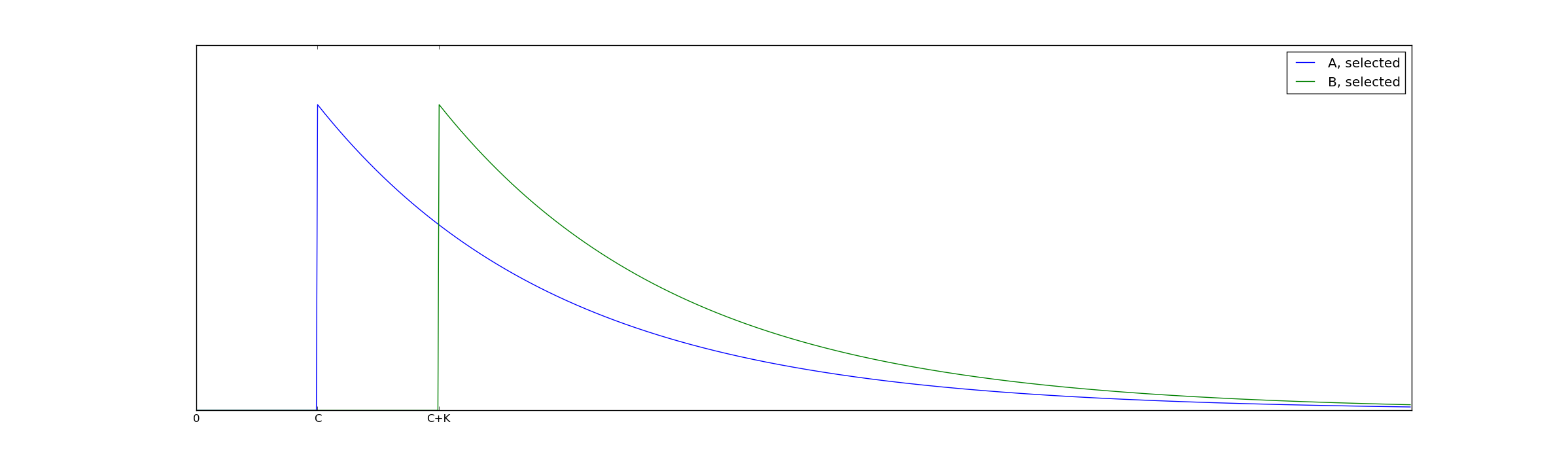
As a result, the mean of the B selected group is higher by the amount $@ K $@ and therefore the decision process is biased against this group by $@ K $@.

Paul Graham's flaw

Unfortunately, using the mean as a test statistic is flawed - it only works when the pre-selection distribution of A and B is identical, at least beyond C. WildUtah on Hacker News came up with a counterexample:

Consider two groups of candidates for a scholarship, A and B. We want to select all candidates that have an 80% or better chance of graduation. Group A comes from a population where the chance of graduation is distributed uniformly from 0% to 100% and group B is from one where the chance is distributed uniformly from 10% to 90%, with the same average but less variation in group B.

Now suppose that we select without bias or inaccuracy all the applicants that have an 80% or better chance of graduation. That means we select a subset of A with a range of 80% to 100% and a subset of B with a range from 80% to 90%. The average graduation rate of scholarship winners from group A will be 90% and that from group B will be 85%.

In pictures, his counterexample looks like this:

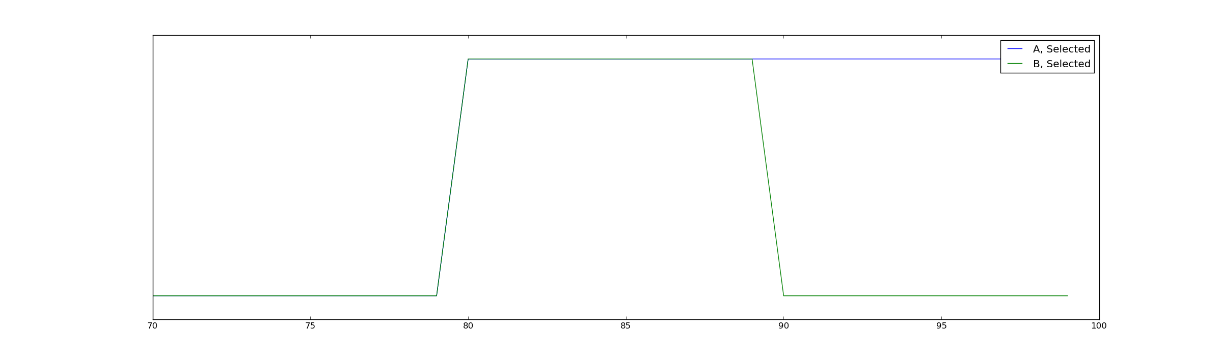
The mean of group B is not lower because of bias (which would be reflected near $@ x=80 $@), but because the very best members of group B are simply not as good as the very best members of group A.

The flaw with Paul Graham's proposed test is the following. His core idea is that bias in favor of group A will cause weak members of group A to be more likely to be accepted than weak members of group B. But the proposed mathematical implementation of this includes both strong and weak members, so it's possible that the effect of strong members might skew the results. Even though the cutoff lives at $@ x = 80 $@, a bunch of group A members with quality 90+ are skewing the average, creating the illusion of bias against A.

Of course, in pictures, it's pretty easy to come up with a possible solution. Rather than trying to measure overall performance, we should instead try to come up with a way to measure marginal performance.

Marginal Performance

The simplest way to look for marginal performance is to try and find the weakest member of each group. In the first graph, the weakest member of group A will be located near \(@ x=C $@ while the weakest member of group B will be located near $@ x=C+K\)@. In the second graph, the weakest member of both groups will be located near $@ x=80 $@.

So rather than comparing mean performance, we'll compare minimum performance.

Our goal now is to try and build a statistical test that encapsulates this idea.

What are the ingredients for a frequentist hypothesis test?

For a frequentist hypothesis test, there are two requirements.

First, we need to have a null hypothesis. In our case, the null hypothesis will be that the selection process is unbiased, and that the minima of both the A and B distributions are identical. We'll assume further that there is a finite and bounded probability of finding elements of A and B near the cutoff. We don't assume we know what the cutoff is.

Once we have the null hypothesis, we need to prove that if the null hypothesis is true, the probability of observing a false positive is bounded. I.e., we need to prove that:

with the property that as $@ \epsilon $@ increases, $@ \delta $@ decreases. This is a bound on the false positive probability of the test, or the probability of type 1 error.

Second, we need an alternative hypothesis. In our case, this will be that the distribution $@ b(x) $@ is supported on an interval $@ [C+K, \infty) $@. Once we have this, we need to prove that:

for some (probably different) $@ \epsilon, \delta $@. This means that if the alternative hypothesis is true, the probability of observing a false negative is bounded.

So what a frequentist hypothesis test does is help distinguish between two possibilities. If the null hypothesis is true, then the test statistic will be close to zero. If the alternative hypothesis is true, then the test statistic should be large.

The test

Now lets take our idea about the world - comparing the weakest member of group A to the weakest member of group B - and translate this into a frequentist hypothesis test. Concretely, let $@ \vec{a} \subseteq A $@ be the A-members who were selected, and $@ \vec{b} \subseteq B $@ be the B-members selected. Then the test statistic is:

Fact 1: In both examples above, this test statistic seems to accurately reflect reality. In my graph, $@ t = -K $@ while in WildUtah's example, $@ t = 0 $@.

In fact, I can prove mathematically that this method is a valid hypothesis test. It will work for any distribution of A and B, provided both sets A and B have a finite probability of having members larger than, but very close to, $@ x=C $@.

So here it is.

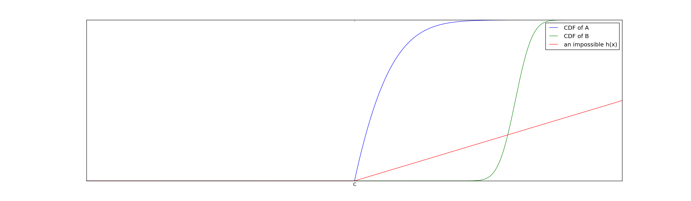
Theorem 1: Take as a null hypothesis the belief that A-members who were selected have the cumulative distribution function $@ a(x) $@ and B-members who were selected have the cdf $@ b(x) $@. Further, we assume that there exists a monotonically increasing function $@ h(0) = 0 $@, $@ 0 \leq h(x), x > 0 $@ such that $@ a(x) > h(x-C) $@ and $@ b(x) > h(x-C) $@. Then assuming this null hypothesis is true, the probability of observing a result at least as extreme as $@ t $@ is bounded above by:

Here \(@N_a\)@ and \(@ N_b\)@ are the number of elements in groups A and B.

Note that it is not necessary to know the value of $@ C $@.

An example of $@ a(x), b(x) $@ and $@ h(x) $@ satisfying the assumptions of Theorem 1 is plotted:

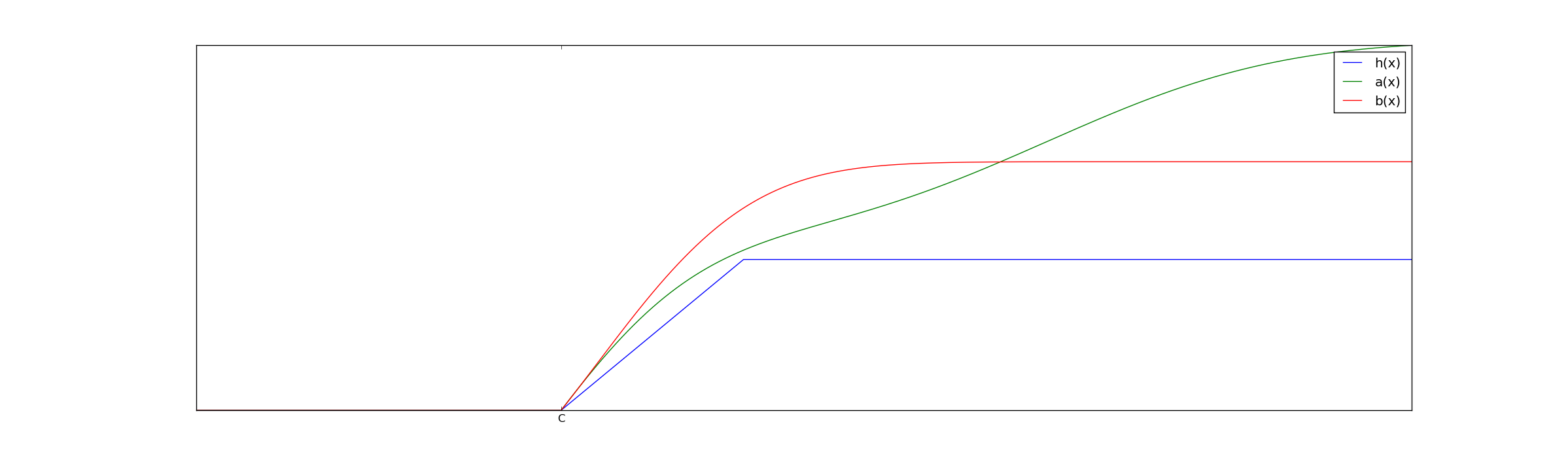
The existence of $@ h(x) $@ simply ensures that both groups have a minimal number of members near the decision boundary $@ C $@.

Proof: The probability of drawing \(@ N_a $@ samples from $@ a(x) $@ and none being contained in $@ [C,C+d/2] $@ is $@ (1-a(C+d/2))^{N_a} \leq (1-h(d/2))^{N_a}\)@, and similarly for $@ b(x) $@ and $@ N_b $@.

Thus, the probability of drawing \(@ N_a\)@ and $@ N_b $@ samples, at least one of which is contained within $@ [C,C+d/2] $@ is bounded below by:

Thus, with probability at least $@ q $@, $@ \min \vec{a} \in [C,C+d/2] $@ and $@ \min \vec{b} \in [C,C+d/2] $@. When this occurs, the test statistic is bounded (in absolute value) by $@d/2 + d/2 = d $@.

Inverting this, we find that with probability at most $@ \hat{p} = 1-q $@, the test statistic $@ t = \min \vec{a} - \min \vec{b} $@ will be larger than $@ d $@. Thus:

is an upper bound on the p-value of the hypothesis test. QED.

Why do we need $@ h(x) $@?

To understand why this assumption that $@ h(x) $@ exists is necessary, consider the following example. Suppose group A is spread out on both the left and right side of the cutoff C, but B is entirely clustered far to the right of the cutoff. For example, see this picture:

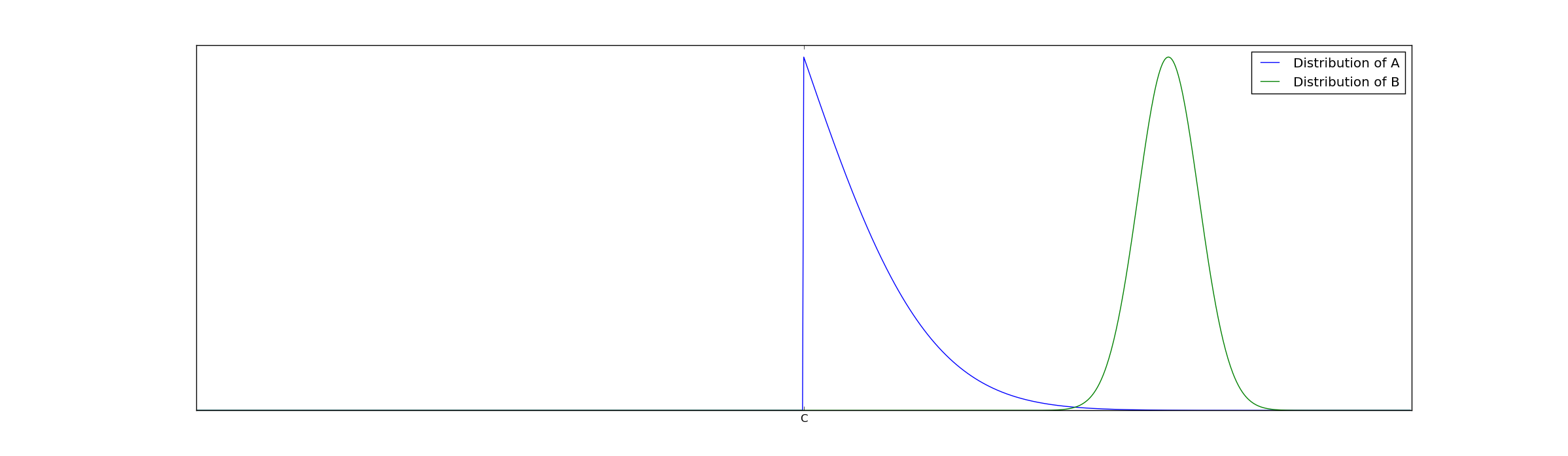
In this case, the statistical test will treat the extreme superiority of group B as bias because every single member of group B exceeds the cutoff.

Our assumption on the existence of $@ h(x) $@ rules out this possibility. If we graph the CDF's of these distributions rather than the PDF, we can pretty easily see why:

Because the green line is zero for a very long distance past the cutoff, $@ b(x) < h(x) $@ in this regime. This violates the assumptions of our statistical test.

In practical terms, distributions like this are rather unrealistic. For example, imagine we want to measure whether colleges are biased against Asians. The examples we describe where no $@ h(x) $@ exists represent the situation where every single Asian person is significantly better than the cutoff. Perhaps a GPA of 3.0 is required to get into college, but every single Asian has a GPA of at least 3.5. Bias is also undetectable here because it has no impact - if Asians are required to have a 3.25 GPA to get into college as compared to a 3.0 for non-Asians, none will ever be rejected due to this bias.

How to use it?

In simple terms, this means that for any probability distributions \(@a(x)\)@ and $@ b(x) $@ which have enough mass near $@ x=C $@, the probability of false positives using this statistical test is bounded. The way one would use this in practice is as follows. First, you'd postulate a specific functional form for $@ h(x) $@. Then you'd run the test, and come up with a $@ t $@ -value. Finally, you could plug this t-value into the formula above.

If the resulting $@ \hat{p} \leq 0.05 $@, then one can safely reject the null hypothesis. Otherwise, one should conclude no evidence for bias.

Concretely, suppose \(@ h(x) = max(x,0) $@. Suppose that we've observed $@ \min \vec{a} = 1.13 $@ while $@ \min \vec{b} = 1.27 $@ with $@N_a=20\)@ and \(@N_b=50\)@.Then:

Thus, we would not reject the null hypothesis. If however we had $@ N_a = 80 $@ and $@ N_b = 200 $@, then $@ \hat{p} = 0.003 $@ and we would reject the null hypothesis, and treat this result as evidence in favor of bias.

Statistical power

We have a similar theorem for statistical power:

Theorem 2: Take as an alternative hypothesis that $@ a(x) $@ is supported in $@ [C,\infty] $@ and is bounded below by $@ h(x) $@ as above. However, suppose that $@ b(x) $@ is supported on $@ [C+K,\infty) $@. Then the probability of a false negative is bounded by:

The proof of this is very simple, so I'll do it right here:

Proof: The only way that $@ t $@ can be smaller than $@ K $@ is if every member of $@ \vec{a} $@ is at least as large as $@ C+K $@. The probability of this occurring is $@(1-a(C+K))^{N_a} \leq (1-h(K))^{N_a} $@. QED.

Given Theorem 2, we now know how to make sure we have enough samples before we start a test. Suppose that (assuming the same functional form of $@ h(x) $@ as above we want a 95% chance of detecting a bias at least as large as $@ K=0.05 $@. Then we want to make:

Equivalently:

Implying:

So this says for us to detect bias at least as large as $@ 0.05 $@ with 95% probability, we need 59 or more samples in each group.

Paul Graham is mathematically wrong, but he did not deserve the criticism he received

Some excerpts of comments from hacker news on Graham's article:

This short comment is not up to pg's usual high standards for his essays.

PG's post was at the level of one of those junk health news articles.

Paul Graham wrote an article about an idea. The idea is generally correct - bias in a decision process will be visible in post-decision distributions, due to the existence of marginal candidates in one group but not the other. But the math was wrong.

That's ok! Very few ideas are perfect when they are first developed. Additionally, I don't think Paul Graham is a statistician. His use of First Round Capital's data (which somehow excluded Uber, and was a tiny sample size) was quite naive - in fact I suspect he only included that example for political reasons (hoping to avoid a repeat of the political attacks he has suffered, perhaps). Then again, most of his critics also didn't understand any stats - quite a few of the critics were making equally egregious mistakes in their desire to jump on the bandwagon.

Paul Graham isn't a statistician, but I am. His idea is solid. Subject to some assumptions (which probably won't be useful to test if VCs are biased), I was able to tweak his idea and get a valid frequentist hypothesis test from it. This new test is also imperfect - it fails to handle noise in measuring inputs/outputs, for example. No statistical test can detect everything, and this one is just something I put together during a very long transatlantic flight.

Any reader is free to criticize me as being "at the level of an evolution denier" or whatever. That's fine, I have a thick skin. But it's also harmful, since some folks don't have a thick skin. Ideas don't spring into the world perfectly formed, with no flaws, ready for immediate use. If we criticize anyone who comes up with a less than perfect idea, we'll just wind up having fewer ideas.

Because I've got a thick skin, any reader is also free to observe flaws and try to fix them. If we don't create disincentives for publicizing and developing imperfect ideas, we'll probably make progress faster.

Also note: As far as handling additive noise, here is where I've gotten stuck. If the tail of the noise is exponential, then I can't figure out how to distinguish between $@ exp(x-C-K) $@ and $@ C exp(x-C) $@. In this case, bias and scaling look the same. Gaussian noise is a lot easier to deal with.

Followup: The paper The Problem of Infra-Marginality in Outcome Tests for Discrimination has been published, which improves these ideas to a version that is actually usable.

Special thanks to Evan Miller and Sidhant Godiwala for reading drafts of this and helping me make it a lot more clear. If you like my post you'll probably also like their blogs. Evan Miller also has suggested his own version of this test - I don't fully understand it, but if we are lucky he'll write about it.

Update: I discovered a paper, The Problem of Infra-Marginality in Outcome Tests for Discrimination which directly addresses this issue. From what I can tell, it's doing a fairly complex hierarchical Bayesian model that's along the same lines as what's described here.