When running a large site, it's important to monitor site behavior. For an ecommerce or similar site, the key thing to measure is conversion rate - if your conversion rate goes down, something is wrong. A common - but wrong - way to measure conversion rate is to simply use a rolling window. If the desired conversion rate is 5%, one might plot the conversion rate over the past 1 hour and trigger an alert if the conversion rate drops below some threshold.
Unfortunately, as Willie Wheeler observes in his blog post Monitoring Bookings and the Law of Large Numbers, a static threshold simply doesn't work. The problem is that variation in the number of visitors over time changes and a reduced number of visitors will increase the variance of your conversion rate. Consider the following scenario - a uniform 5% conversion rate. During some time periods the number of visitors is 10,000, while during others it's only 1,000.
Supose we were to raise an alert whenever the empirical conversion rate dropped below 4%. In this case, the false positive rate during periods when there are 10,000 visitors would be only binom(10000, 0.05).cdf(400) == 1.21e-06. That's pretty good! However, during the low traffic periods, that false positive rate rises to binom(1000, 0.05).cdf(40) = 0.081. Whoops!
In pictures, here's what happens:
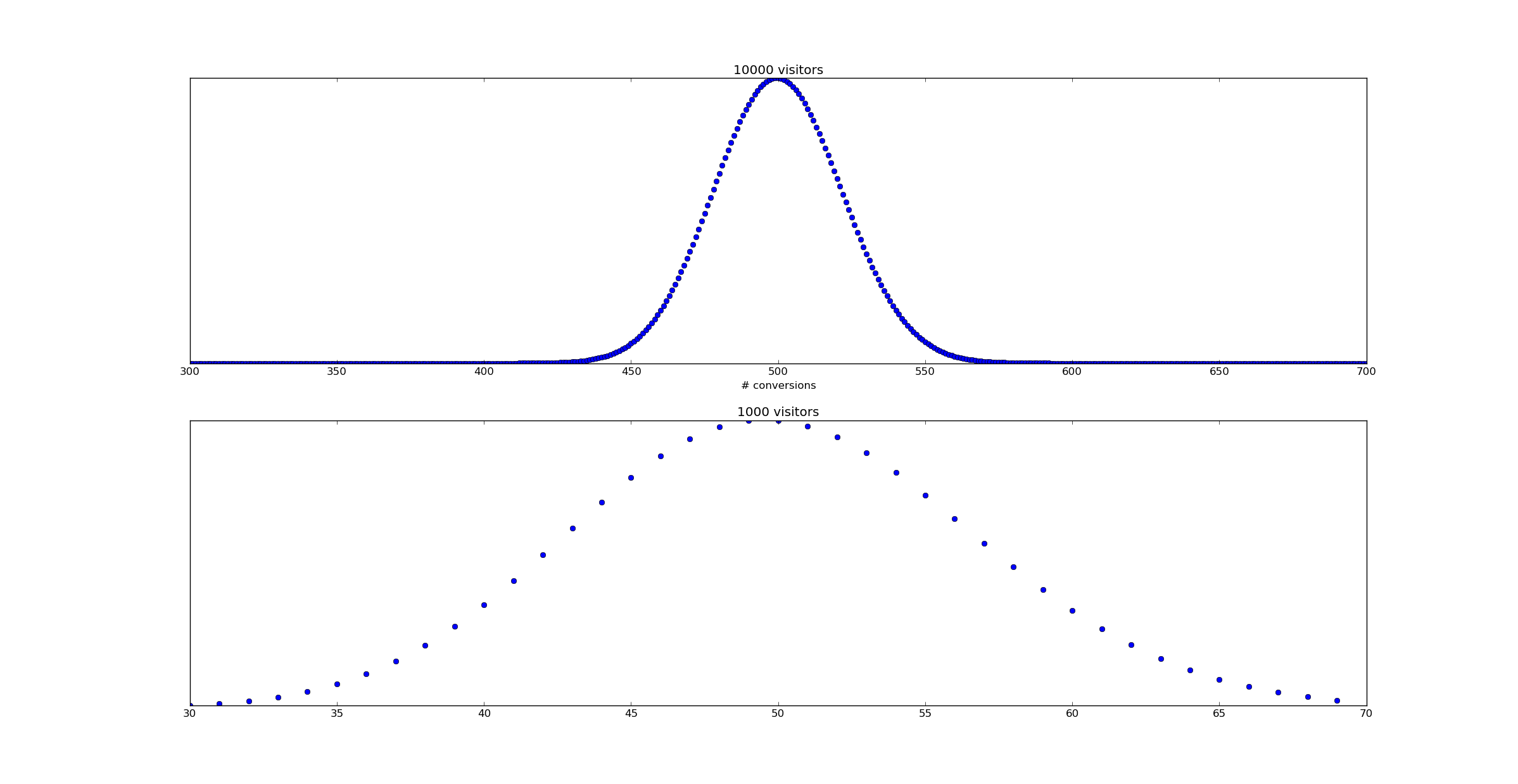
Based on this analysis it's pretty clear no static threshold can be used - a tight threshold for the 10,000 visitor time periods would have a huge number of false positives for the 1,000 visitor case.
This problem can be resolved by a Bayesian timeseries model.
Bayesian Timeseries Analysis
A timeseries is simply a function of time - $@ f: \mathbb{R} \rightarrow T $@. Bayesian timeseries analysis is simply the discipline of using Bayesian statistics to study functions which vary (possibly stochastically) with time. As an example, lets consider how the problem of monitoring conversion rate over time can be framed as a statistics problem.
Here's the basic idea. Let us allow $@ \theta(t) $@ to reprsent our conversion rate as a function of time. As an oversimplified model, lets assume $@ \theta(t) $@ takes the following form. First of all, at $@ t = 0 $@, $@ \theta(t) = p_0 $@. As time progresses, the conversion rate can change instantaneously at a known average rate $@ \lambda $@ per unit time. Supposing the conversion rate changes at time $@ t_1 $@, it will change to a new rate $@ p_1 $@ drawn from a known distribution $@ f(p) $@.
So in simple terms:
If we could measure \(@ \theta(t) $@ directly, it would be straightforward to identify $@p_0\)@, \(@p_1\)@ and $@ t_1 $@. And if we have enough data (say 10,000 data points per unit of time), we can easily observe this:
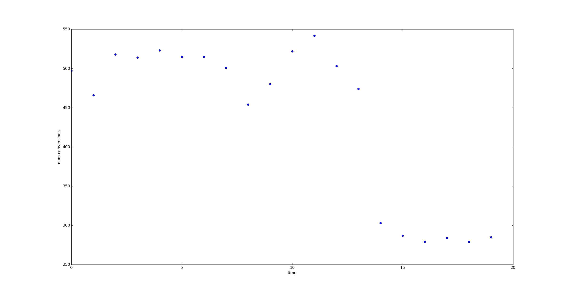
But when the number of data points we have is lower - say 1,000 per unit time - it's harder to observe a jump.
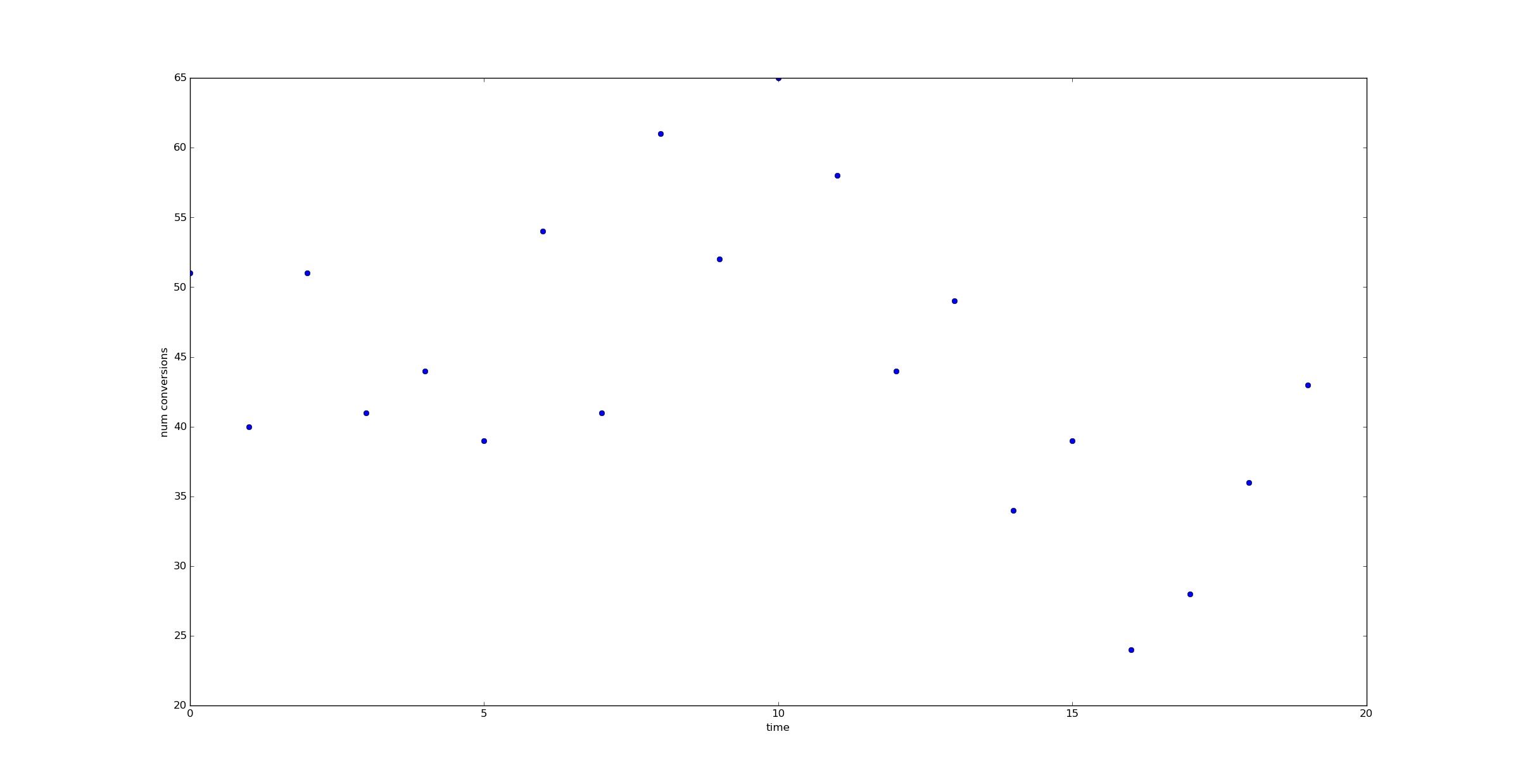
How can we extract the maximal amount of information from the data available?
Computing the likelihood of a timeseries
Consider a timeseries $@ \theta(t) $@. Suppose we've made an observation - at time $@ t $@ there were $@ n_t $@ visitors and $@ c_t $@ conversions. What is the likelihood that this occurred?
The likelihood is defined as $@ P(c_t | \theta(t), n_t) $@. It's the probability of seeing the result we just saw, given some value of the unknown parameter. Luckily this question is easily answered with the Binomial theorem:
Now given a data series - a sequence of points $@ (n_1, c_1), (n_2, c_2), \ldots $@, we can compute the likelihood of observing this series:
Sometimes more usefully, we might wish to consider the log likelihood:
Computing the likelihood with Python
Suppose now we have input data - a timeseries n and c representing visitor count and conversions:
n = array([ 1000.,  1000.,  1000.,  1000.,  1000.,  1000.,  1000.,  1000.,
            1000.,  1000.,  1000.,  1000.,  1000.,  1000.,  1000.,  1000.,
            1000.,  1000.,  1000.,  1000.])

c = array([51, 40, 51, 41, 44, 39, 54, 41, 61, 52, 65, 58, 44, 49, 34, 39, 24,
           28, 36, 43])
Then let us represent theta with an array as well.
theta = array([ 0.05,  0.05,  0.05,  0.05,  0.05,  0.05,  0.05,  0.05,  0.05,
                0.05,  0.05,  0.05,  0.05,  0.05,  0.05,  0.05,  0.05,  0.05,
                0.05,  0.05])
The log likelihood can be computed via:
def log_likelihood(n, c, theta):
    return sum(binom.logpmf(c, n, theta))
And of course the likelihood itself can be computed via:
def likelihood(n, c, theta):
    return exp(log_likelihood(n,c,theta))
Comparing likelihoods
Now let us imagine we had two alternate theories about what $@ \theta(t) $@ might be. Consider our first hypothesis - a sort of a "null hypothesis" - as the theory that the conversion rate has remained constant:
Now consider an "alternate hypothesis" - the assumption that the conversion rate dropped from 5% to 3% at time 14.
This is a very specific alternate hypothesis (it's exactly how I generated the data) which I'm choosing for illustrative purposes. I put "null hypothesis" and "alternate hypothesis" in scare quotes since I'm not planning on using them in a Frequentist manner.
Using the likelihood formula for $@ P(c_1, c_2, \ldots | \theta(t), n_1, n_2, \ldots) $@ above, we find that:
and
(I've shifted to a log scale to make the numbers easier to observe.)
Now lets consider a range of alternate hypothesis, each representing the possibility of a jump at a different time:
We can plot the log likelihood of these various alternate hypothesis. The green line in this plot represents the "null hypothesis" that no jump occurred, and the conversion rate remained 5% for all time.
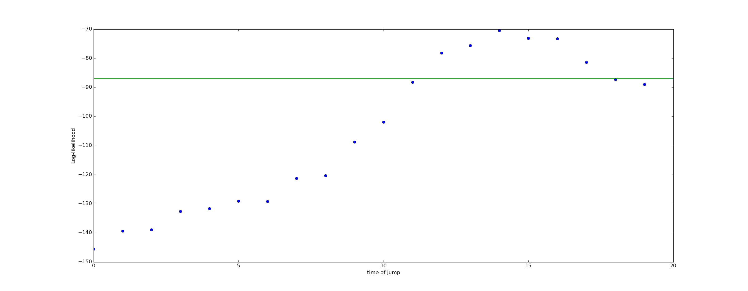
The fact that the log likelihood peaks at $@ t=14 $@ suggesting that whatever we believed before, we should hold a stronger belief that our conversion rate dropped from 5% to 3% at approximately $@ t = 14 $@.
Bayesian Inference
Bayesian inference takes our rough intuition - that we should consider a drop in conversion rate at $@ t = 14 $@ to be more likely than before - and quantifies it.
To do Bayesian inference, we need to come up with a prior. As a prior, I'll assume that a drop in conversion rate is unlikely - only 2%. I'll also assume that the probability of a drop occurring at any given time is equal.
For simplicity I'll assume that if a drop occurs, the drop is from 5% to 3%.
Thus, as a prior, we obtain:
To compute a posterior, we need to use Bayes rule:
So for example, we can compute the probability of there being no jump as:
In contrast, the probability of a jump at t=14 is:
Repeating this calculation for all times yields the following plot of the posterior on the time at which the conversion rate dropped:
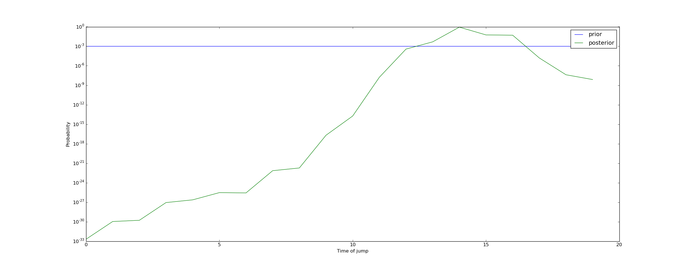
We can draw the conclusion that a jump almost certainly occurred (with probability 99.95%) at some point between t=13 and t=17. This means we should raise an alert!
Doing the calculation in Python
The following code implements the computation of the posterior:
from pylab import *
from scipy.stats import binom

def log_likelihood(n, c, theta):
    return sum(binom.logpmf(c, n, theta))

def bayesian_jump_detector(n, c, base_cr=0.05, null_prior=0.98, post_jump_cr=0.03):
    """ Returns a posterior describing our beliefs on the probability of a
    jump, and if so when it occurred.

    First return value is probability null hypothesis is true, second return
    value is array representing the probability of a jump at each time.
    """
    theta = full(n.shape, base_cr)
    likelihood = zeros(shape=(n.shape[0] + 1,), dtype=float) #First element represents the probability of no jump

    likelihood[0] = null_prior #Set likelihood equal to prior
    likelihood[1:] = (1.0-null_prior) / n.shape[0] #Remainder represents probability of a jump at a fixed increment

    likelihood[0] = likelihood[0] * exp(log_likelihood(n, c, theta))
    for i in range(n.shape[0]):
        theta[:] = base_cr
        theta[i:] = post_jump_cr
        likelihood[i+1] = likelihood[i+1] * exp(log_likelihood(n, c, theta))
    likelihood /= sum(likelihood)
    return (likelihood[0], likelihood[1:])
Experiments with other scenarios
If we now consider a situation with only 100 visitors/time unit, we can run this code as well.
n = full((20,), 100)
c = binom(100, 0.05).rvs(20) #No jump in CR occurs

bayesian_jump_detector(n, c, null_prior=0.99)

#Result is:
(0.99888216914806816,
 array([  7.28189038e-11,   2.20197564e-10,   6.65856870e-10,
          2.40083185e-10,   4.26612169e-10,   1.29003536e-09,
          7.91551819e-10,   1.40653598e-09,   7.23795867e-09,
          6.33837938e-08,   1.91666673e-07,   1.17604609e-07,
          1.22800167e-07,   3.71336237e-07,   3.87741199e-07,
          6.88990834e-07,   3.54550985e-06,   1.82450034e-05,
          2.71896088e-04,   8.22188376e-04]))
In this case, our confidence in the null hypothesis has increased from 99% to 99.89%.
What if we put a jump in?
n = full((20,), 100)
c = binom(100, 0.05).rvs(20)
c[13:] = binom(100, 0.03).rvs(7) #Jump occurs at t=13

bayesian_jump_detector(n, c, null_prior=0.99)

#Result is:
(0.92236200077388664,
 array([  2.78977290e-06,   2.91302001e-06,   5.17624665e-06,
          2.66366875e-05,   1.37070964e-04,   8.41052693e-05,
          8.78208876e-05,   2.65562162e-04,   9.57518240e-05,
          9.99819660e-05,   1.04398988e-04,   5.37231589e-04,
          4.70461049e-03,   4.11989173e-02,   1.48547950e-02,
          9.11474243e-03,   1.93120502e-03,   2.01652216e-03,
          2.10560845e-03,   2.62158967e-04]))
Because in this case we have a lot less data (100 data points/time unit vs 1000), we do not have as much confidence in our result. Our belief in the null hypothesis has dropped from 99% to 92%, and our belief that a drop has occurred near t=13 has increased to about 6% (with the remaining 2% spread out a little further). That's enough to raise an alert, but not enough to conclusively determine that the effect is real.
Conclusion
Bayesian timeseries analysis is just ordinary Bayesian statistics, but we are doing our analysis in a space of functions. Our goal is to characterize probabilistically an unknown function $@ \theta(t) $@ which generates one or more observable data series, e.g. $@ n_t, c_t $@. In this post I've discussed anomaly detection, but this is actually a very general mode of thinking which can be used under a lot of circumstances.
In particular, I hope in a later post to comment on time varying conversion rates. Specifically, in another post on his blog, Willie Wheeler discusses the issue of time periodic conversion rates. I.e., the assumption here is that absent a negative downward spike, $@ \theta(t) $@ should be time periodic - Tuesday and Saturday differ, but last Tuesday is a lot like this Tuesday. With some luck I'll come back to this topic, and discuss how to handle such situations in a Bayesian formulation.