In a previous job, I built a machine learning system to detect financial fraud. Fraud was a big problem at the time - for simplicity of having nice round numbers, suppose 10% of attempted transactions were fraudulent. My machine learning system worked great - as a further set of made-up round numbers, lets describe it as having a precision and recall of 50% each. All this resulted in a fantastic bite taken out of the fraud problem.
It worked so well that fraud dropped by well over 50% - because of the effort involved in getting past the system, fraudsters just gave up and stopped trying to scam us.
Suddenly the system's performance tanked - recall stayed at 50% but precision dropped to 8%! After some diagnosis, I discovered the cause was the following - all the fraudsters had gone away. For every fraud attempt, the system had a 50% chance of flagging it. For every non-fraudulent transaction, the system had a 5.5% chance of flagging it.
Early on, fraud attempts made up 10% of our transactions. Thus, for every 1000 transactions, we would flag 50 of the 100 fraudulent transactions and 50 of the 900 good transactions. This means that for every 10 flags, 5 are correct - hence a precision of 50%.
Once the fraudsters fucked off, fraud attempts dropped to perhaps 1% of our transactions. For every 1000 transactions, only 10 were fraudulent. We would flag 5 of them, along with 5.5% x 990 legitimate transactions = 54 transactions. The net result is that only 5 of the 59 transactions we flagged as fraudulent actually were, for a precision of 8%.
This phenomenon is called label shift. The problem with label shift is that the base rate for the target class changes with time and this significantly affects the precision of the classifier.
Typical characteristics of the problem
In general, the following are characteristics of the problem that I'm generally interested in:
- \(N\) not too large - potentially under 100k.
- \(\alpha\) in the ballpark of 0.1% to 5%.
These kinds of problems are typical in security, fraud prevention, medicine, and other situations of attempting to detect harmful anomalous behavior.
Precision, Risk Thresholds and Loss Functions
For most classifiers the ultimate goal is to make a decision. The decision is taken in order to minimize some loss function which represents the real world cost of making a mistake.
Consider as an example a clasifier \(f: \mathbb{R}^K \rightarrow \mathbb{R}\) used to predict a disease. Let us define \(\vec{x} \in \mathbb{R}^K\) to be our feature vector, \(z \in [0,1]\) to be our risk score and \(y \in 0,1\) whether or not the patient actually has the disease.
A loss function might represent the loss in QUALYs from making an error. Concretely, suppose that a failure to diagnose a disease results in the immediate death of the patient - this is a loss of 78 - patient's age QUALYs. On the flip side, treatment is also risky - perhaps 5% of patients are allergic and also die instantly. This is a loss of 5% x (78 - patient's age) [1]. Represented mathematically, our loss function is:
Let us also suppose that we have a calibrated risk score, i.e. a monotonically increasing function \(c: [0,1]->[0,1]\) with the property that \(c(z)=P(y=1|z)\). For a given patient, the expected loss from treatment is therefore:
while the loss from non-treatment is:
The expected loss from treatment exceeds the expected loss from non-treatment when \(c(z) > 0.05/1.05 \approx 0.0526\), so the optimal decision rule is to treat every patient with a (calibrated) risk score larger than 0.0526 while letting the others go untreated.
The effect of label shift on calibration
Let's study this from the perspective of score distributions. Suppose that \(f_0(z)\) is the pdf of the distribution \(z | y=0\) and \(f_1(z)\) is the pdf of the distribution \(z | y=1\). For simplicity, assume these distributions are monotonic.
Suppose now that the base rate is \(P(y=1)=\alpha\). In this framework, a label shift can be represented simply as a change in \(\alpha\).
It is straightforward to calculate the calibration curve (as a function \(\alpha\)) as:
As is apparent from this formula, a change in \(\alpha\) will result in a change in calibration. The following graph provides an example:
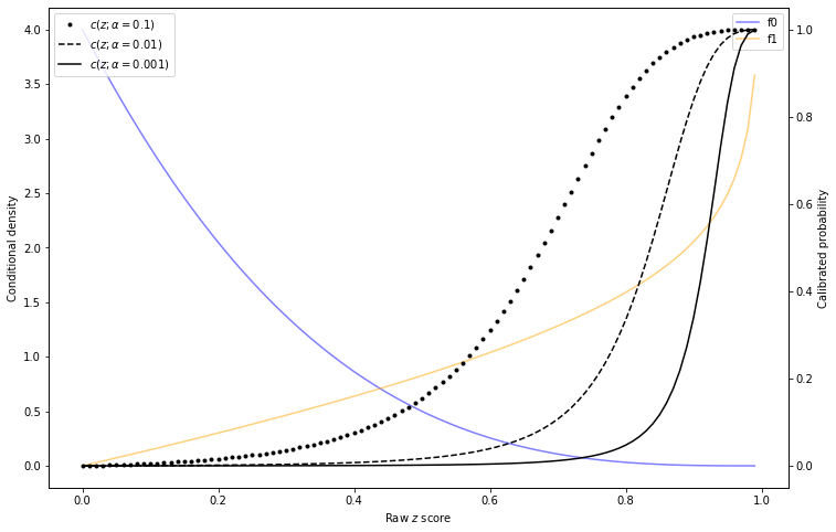
Illustration of calibration curves changing with base rate
Let's consider the effect of this on decisionmaking. Going back to our disease example above, suppose that at model training/calibration time, \(\alpha=0.01\). Then a disease outbreak occurs and \(\alpha=0.1\). The decision rule being used based on the training data (with \(\alpha=0.01\)) says to treat any patient with raw \(z\) score of 0.65 or greater.
But once \(\alpha=0.1\), the actual infection probability of a person with \(z=0.65\) is nearly 40%. As per the loss function calculation earlier, we want to treat any patient with a 5.26% or greater chance of being sick!
In the literature, when making batch predictions, there's a known technique for solving this (see discussion [2]). The basic idea is the following. For a set of raw risk scores \(z_i, i=1\ldots N\), we know they are drawn from the distribution:
Thus, one can estimate \(\alpha\) via the maximum likelihood principle (although the literature describes a slightly different approach [3]):
Maximizing this is straightforward - take logs, compute \(\frac{\partial L}{\partial \alpha}\), use scipy.optimize.minimize.
What happens when the distribution changes?
The method described above is strongly sensitive to the assumption that the shape of the distribution of the positive class \(f_1(z)\) does not change, only it's amplitude \(\alpha\).
However in practice, we often discover that \(f_1(Z)\) changes with time as well. For example, consider again the example of disease prediction - a new strain of a known disease may have a somewhat different symptom distribution in the future than in the past. However it is a reasonable assumption to make that the shape of \(f_0(z)\) remains the same; healthy people do not change their health profile until they become infected.
Thus, the more general situation I'm considering is a mix of label shift/base rate changes, together with small to moderate changes in the distribution of the exceptional class only. By "exceptional class", I mean "sick" (in disease prediction), "fraud" (in fraud prevention), essentially the uncommon label which corresponds to something anomalous.
In general, it is impossible to solve this problem [5]. However, if we stay away from this degenerate case (see footnote [5]), it's actually quite possible to solve this problem and estimate both the new shape of \(f_1(z)\) and \(\alpha\). The main restriction is that \(f_1(z)\) is not too different from the old value, but right now I don't have a good characterization of what "not too different" actually means.
Formal statement of the setup
In the training phase, we have a labelled data set \((\vec{x}_i, y_i), i=1\ldots N\) on which we can train any sort of model that generates risk scores \(z_i, i=1 \ldots N\). We will assume that in this data set, the risk scores \(z_i\) are drawn from \(f_0(z)\) if \(y_i=0\) and \(f_1(z)\) if \(y_i=1\).
In the prediction phase we will consider batch predictions. We receive a new set of \(\vec{x}\) and we can of course use the already trained classifier to generate risk scores \(z_i\). Our goal is for each data point \(z_i\) to generate a calibrated risk score \(c(z_i) \approx P(y_i=1|z_i)\).
Without label shift there is a standard approach to this that is implemented in sklearn as sklearn.calibration.CalibratedClassifierCV. Typically this involves running isotonic regression on a subset of the training data and the mapping \(c(z)\) is the result of this.
That does not work in this case because \(c(z)\) computed in the training phase will be for the wrong distribution. The figure Illustration of calibration curves changing with base rate illustrates this - isotonic calibration may correctly fit the curve \(c(z; \alpha=0.01)\) in the training phase. But if the right curve in the prediction phase is \(c(z; \alpha=0.1)\), that fit is not actually correct. This blog post aims to address that problem.
My method
The approach I'm taking is upgrading the maximum likelihood estimation to a max-aposteriori estimation.
I first parameterize the shape of the exceptional label \(f_1(z;\vec{q})\) with \(\vec{q} \in \mathbb{R}^m\). I then construct a Bayesian prior on it which is clustered near \(f_1(z)\). It is straightforwardly derived from Bayes rule that x:
For simplicity I'm taking \(P(\alpha, \vec{q}) = P(\vec{q})\), a uniform prior on \(\alpha\).
Once the posterior is computed, we can replace maximum likelihood with max-aposteriori estimation. This provides a plausible point estimate for \((\alpha, \vec{q})\) which we can then use for calibration.
Kernel Density Estimation on [0,1]
The first step is doing kernel density estimation in 1-dimension in a manner that respects the domain of the function. Gaussian KDE does NOT fit the bill here because the support of a gaussian kernel is \(\mathbb{R}\), not \([0,1]\). One approach (which is somewhat technical and I couldn't make performant) is using beta-function KDE instead [4]. An additional technical challenge with using traditional KDE approaches on this problem is that whatever approach is taken, it also needs to be fit into a max-likelihood/max-aposteriori type method.
I took a simpler approach and simply used linear splines in a manner that's easy to work with in scipy. Suppose we have node points \(\zeta_0=0, \zeta_1, \ldots, \zeta_m=1\). Then let us define the distribution \(f_1(z; \vec{q})\) as a normal piecewise linear function:
for \(z \in [\zeta_k,\zeta_{k+1}]\) with \(h_i\) defined as
and
I chose this parameterization because scipy.optimize.minimize doesn't do constrained optimization very well. With this parameterization, all values \(\vec{q} \in \mathbb{R}^m\) yield a valid probability distribution on \([0,1]\).
Python code implementing this is available in the linked notebook, implemented as PiecewiseLinearKDE. Calculations of \(\nabla_{\vec{q}} h_i(\vec{q})\) - used in numerical optimization - can also be found in that notebook. Most of it is straightforward.
Fitting a piecewise linear distribution to data is only a few lines of code:
from scipy.optimize import minimize
def objective(q):
    p = PiecewiseLinearKDE(zz, q)
    return -1*np.log(p(z)+reg).sum() / len(z)

def deriv(q):
    p = PiecewiseLinearKDE(zz, q)
    return -1*p.grad_q(z) @ (1.0/(p(z)+reg)) / len(z)

result = minimize(objective, jac=deriv, x0=np.zeros(shape=(len(zeta)-1,)), method='tnc', tol=1e-6, options={'maxiter': 10000})
result = PiecewiseLinearKDE(zeta, result.x)
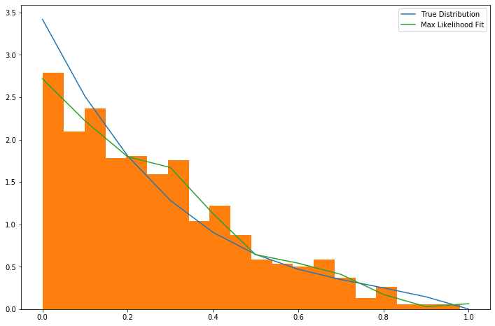
The result is approximately what one might expect.
One useful coding trick to take away from this is our use of np.interp inside a number of methods of PiecewiseLinearKDE. Since the curve itself is computed as np.interp(x, self.nodes, self.h()), gradients of this w.r.t. q can then then be computed by applying np.interp(x, self.nodes, grad_h) where grad_h is the gradient of \(\vec{h}\) w.r.t. \(\vec{q}\). This then allows the efficient calculation of gradients of likelihood functions as seen in deriv above, simplifying what might otherwise be index-heavy code.
Computing a posterior and max-aposteriori estimation
Defining a prior on a function space - e.g. the space of all probability distributions on [0,1] - is not a simple matter. However, once we've chosen a parameterization for \(f_1(z; \vec{q})\), it becomes straightforward. Since \(\vec{q} \in \mathbb{R}^m\), the restriction of any reasonable prior onto this space is absolutely continuous w.r.t. Lebesgue measure, thereby eliminating any theoretical concerns.
The situation we are attempting to model is a small to moderate change in the distribution of \(f_1(z)\), particularly in regions where \(f_0(z)\) is small. So we will define the (unnormalized) prior to be:
where \(g(x) = \sqrt{1+x^2}-1\) is a basically just a smoothed out (differentiable) version of \(|x|\). We need a smooth version of \(|x|\) simply because when we do max-aposteriori later, a smooth curve makes numerical minimization easier.
This prior should not be thought of as a principled Bayesian prior, but merely one chosen for convenience and because it regularizes the method. If we ignore the smoothing, this is analogous to a prior that penalizes deviation from \(f_1(z)\) in the \(L^p(f_0(z) dz)\) metric. The measure \(f_0(z) dz\) is used to penalize deviation more in areas where \(f_0(z)\) is large. The parameter \(\beta\) represents the strength of the prior - larger \(\beta\) means that \(f_1(z; \vec{q})\) will remain closer to \(f_1(z)\).
One important note about the power \(p\). Because \(g(x) = O(x^2)\) as \(x \rightarrow 0\), choosing \(p=1\) does NOT actually generate any kind of sparsity penalty, in contrast to using \(|x|^1\).
The likelihood is (as per the above):
Computing the log of likelihood times prior (neglecting the normalization term from Bayes rule), we obtain:
The gradient of this with respect to \((\alpha, \vec{q})\) is:
Using this objective function and gradient, it is straightforward to use scipy.optimize.minimize to simultaneously find both \(\vec{q}\) and \(\alpha\).
Examples
Note: All of the examples here are computed in this Jupyter notebook. For more specific details on how they were performed, the notebook is the place to look.
Here's an example. I took a distribution of 97.7% negative samples, with a relatively simple prior distribution. I simulated a significant change of shape in the distribution of \(z\) scores of the positive class, which is illustrated in red in the graph below. As can be seen, the approximation (the orange line) is reasonably good. Moreover, we recover \(\alpha\) with reasonable accuracy - the measured \(\alpha\) was 0.0225 while the true \(\alpha\) was 0.0234.
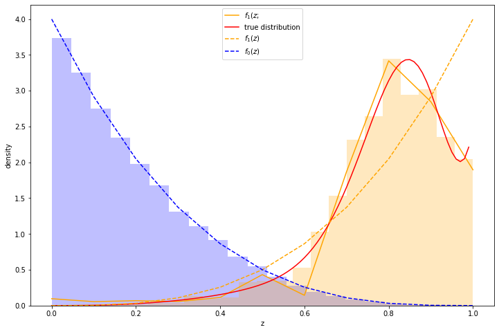
(The histograms in the graph illustrate the actual samples drawn.)
Using the fitted curve to compute calibration seems to work reasonably well, although simple isotonic regression is another way to do it.
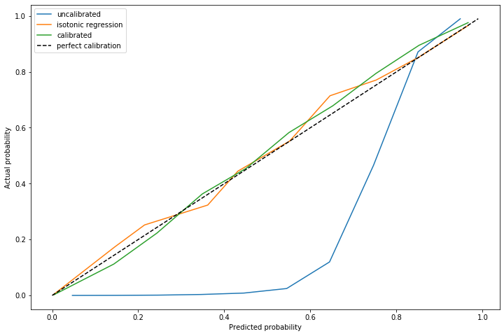
The advantage of using this method is on out of sample data with a significantly different distribution of positive cases. I repeated this experiment, but with \(\alpha=0.011\) and a marginally different distribution of positive cases.
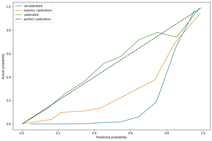
The dynamically calculated calibration curve (the green) still behaves well, while the isotonic fit calculated for a different \(\alpha\) (unsurprisingly) does not provide good calibration.
Note that recalculating the isotonic fit is not possible, since that requires outcome data which is not yet available.
Estimating Bayes loss
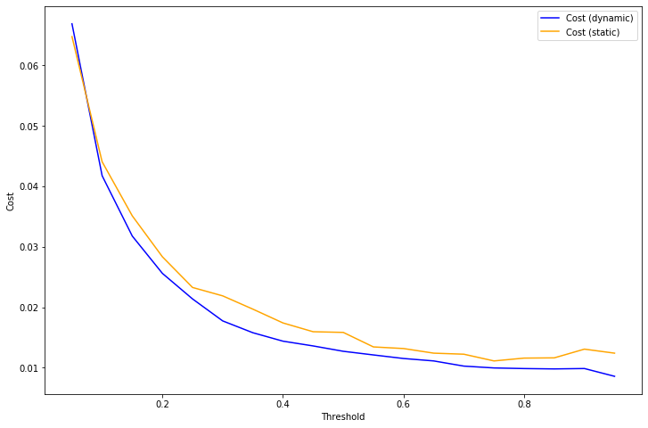
The major use case for this method of calibration is reducing the loss of a decision rule due to model miscalibration. Consider a loss function which penalizes false positives and false negatives. Without loss of generality [6], such a loss function takes this form:
With this loss function, the optimal decision rule is to choose 1 (positive) whenever \(c(z) >= T\), otherwise choose 0 (negative).
Using the same example as above, we can compute the result of applying this decision rule using either isotonic calibration (static) or our dynamic rule to the test set. For almost every choice of threshold \(T\), the loss is significantly lower when using the dynamic calibration.
Other metrics
A method such as this should NOT be expected to improve ROC_AUC, and in fact in empirical tests this method does not. This is because ROC_AUC is based primarily on ordering of risk scores, and our calibration rule does not change the ordering.
The Brier Score - an explicit metric of calibration - does tend to increase with this method. This is of course completely expected. In my experiments, this method is less effective at generating a low Brier score than Isotonic calibration at least until either \(\alpha\) or \(\vec{q}\) changes.
The average precision score also tends to increase over multiple batches with different \(\alpha, \vec{q}\).
Comparison to more standard label shift methods
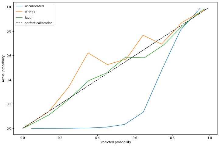
Another approach (the approach of papers linked in footnote [2]) is to simply fit \(\alpha\) and do not allow \(f_1(z)\) to change.
In experiments, I've noticed that fitting \(\alpha\) without allowing \(f_1(z)\) to change generally produces a more accurate estimate of \(\alpha\), even in situations where the true distribution differs significantly from \(f_1(z)\).
However, in spite of a more accurate estimate of \(\alpha\), the resulting calibration curves from fitting only \(\alpha\) do not tend to be as accurate. The curve that comes from fitting \(\alpha, \vec{q}\) is more accurate than the fit of \(\alpha\) alone:
Future work
At this stage I do not consider this method in any sense "production ready". I do not have a great grasp on the conditions when this method works or fails. I've also observed that very frequently, scipy.optimize.minimize fails to converge, yet returns a useful result anyway. Most likely I'm looking for too high a tolerance.
I've also tried a couple of other ways to parameterize the probability distributions and the method seems quite sensitive to them. For example, I included an unnecessary parameter in an earlier variation - \(h_0=e^{q_0}/M(\vec{q})\) - and this completely caused the method to fail to converge. I'm not entirely sure why.
There is a corresponding Jupyter notebook which has the code to do this this. If anyone finds this useful and is able to move it forward, please let me know! As a warning, playing around with the code in the notebook will make the warts of the method fairly visible - e.g. once in a while, a cell will fail to converge, or just converge to something a bit weird.
However, overall I am encouraged by this. I believe it's a promising approach to dynamically adjusting calibration curves and better using prediction models in a context when the distribution of the positive class is highly variable.
Active learning
As one additional note, I'll mention that I have some work (which I'll write about soon) suggesting that if we can request labels for a subset of the data points, we can do reasonably efficient active learning of calibration curves. This appears to significantly improve accuracy and reduce the number of samples needed.
Notes
| [1] | In reality 78 should be replaced with life expectancy at the time of diagnosis, which is typically larger than the mean population life expectancy. This is a technical detail irrelevant for this post. |
| [2] | (1, 2, 3) Adjusting the Outputs of a Classifier to New a Priori Probabilities: A Simple Procedure, by Marco Saerens, Patrice Latinne & Christine Decaestecker. Another useful paper is EM with Bias-Corrected Calibration is Hard-To-Beat at Label Shift Adaptation which compares the maximum likelihood method with other more complex methods and finds it's generally competitive. This paper also suggests max likelihood type methods are usually the best. |
| [3] | The approach taken in the papers cited in [2] are a bit different - they do expectation maximization and actually generate parameters representing outcome variables, requiring use of expectation maximization. The approach I'm describing just represents likelihoods of z-scores and ignores outcomes. But in principle these approaches are quite similar, and in testing the version I use tends to be a bit simpler and still works. |
| [4] | Adaptive Estimation of a Density Function Using Beta Kernels by Karine Bertin and Nicolas Klutchnikoff. |
| [5] | (1, 2) Suppose that the distribution \(f_1(z)\) changes so that \(f_1(z)=f_0(z)\). Then for all \(\alpha_0, \alpha_1 \in [0,1]\), \([(1-\alpha_0)f_0(Z) + \alpha_0 f_1(Z)] \equiv [(1-\alpha_1)f_0(Z) + \alpha_1 f_1(Z)]\) and therefore it is impossible to distinguish between different values of \(\alpha\) from the distribution of \(z\) alone. |
| [6] | Suppose we had an arbitrary loss function with a false positive cost of \(A\) and a false negative cost of \(B\). Then define \(T=(A/B)/(1+A/B)\) and \(C=BT\). This is equivalent to a loss function with penalties \(C/(1-T)\) for false positives and \(C/T\) for false negatives, which differs from our choice of loss function only by a multiplicative constant \(C\). |