How to measure a changing conversion rate (with python code)

As the owner of the spamblog http://www.iwishiwastaller.com, I've run into the following problem. I'm selling some height enhancing pills full of organic free range snake oil. I've come up with several different calls to action:

Tired of finding pants that fit? Click here for the solution.
Click here if you find airplane seats too comfortable.
The NBA hates him! Click here to learn one weird trick for becoming taller!

For obvious reasons, my first thought was to try an A/B test to figure out the best one. It gave me an answer - "one weird trick" was the winner. But just out of curiosity, I ran the test again the next day and discovered that "Tired of finding pants that fit" was the winner. Curious now, I repeated my test several more times, and discovered that the best version changed over time!

This is a problem. A/B testing cannot find the best call to action, nor can traditional bandit algorithms. Most statistical techniques for estimating the conversion rate all assume it remains constant. So to solve this problem, I need to come up with a new method. In this blog post I'll provide a Bayesian statistical technique that can estimate a conversion rate which changes with time. In later blog posts I'll actually discuss how to use this for conversion rate optimization.

Background expected: I'm aiming this blog post at people who know at least basic probability and some coding. For a background on the relevant probability, go read the blog post Analyzing conversion rates with Bayes Rule. I include a few differential equations in this post. If you don't understand them, ignore them and just keep reading. Since I know most of my readers are coders rather than mathematicians, after every equation I include some python code to illustrate what the equation means.

The Model

To simplify the discussion I'll focus solely on the conversion rate of a single call to action. Call this rate $@X=X_t$@, where $@t$@ is time. The value $@X_t$@ denotes the probability that at time $@t$@, a display of the call to action will result in a conversion.

I will assume that the conversion rate $@X_t$@ follows a random walk. For mathematical simplicity I'll choose a standard model called Jacobi Diffusion. Jacobi diffusion is makes two assumptions about the click through rate. The first is that over time, the click through rate approaches a fixed value. The second assumption is that in addition to approaching a fixed value, the click through rate also moves around randomly.

The nature of the randomness is chosen with a weighting parameter - specifically, the closer the CTR gets to 0 or 1, the smaller the random movements become. This is done to ensure that the CTR never becomes larger than 1 or smaller than 0, which would obviously make no sense.

The mathematical model I choose is:

$$ d x_t = - \frac{1}{2}\theta \left((2 X_t-1) - \frac{b-a}{a+b+2} \right) dt + \frac{1}{2}\sqrt{ \frac{\theta}{2(a+b+2)} X_t(1-X_t) } dW_t $$

In this equation, $@ dW_t $@ is a brownian motion term.

For those more familiar with python code than differential equations, I could represent it as:

gaussian_var = norm() # a normal distribution
dt = 0.01 # or other small value - this is the timestep
tmax = 3 # or some other large value - this is the maximum time i am interested in
x = zeros(shape=(int(tmax/dt),), dtype=float)
x[0] = initial_CTR

for i in range(1, x.shape[0]):
    x[i] = x[i-1]
             - (theta/2)*(2*x[i-1]-1 - (b-a)/(a+b+2))*dt
             + 0.5*sqrt((theta/(2*(a+b+2)))*x[i-1]*(1-x[i-1]))*gaussian_var.rvs()*sqrt(dt)

So at each timestep the CTR approaches it's mean value (due to the term - (theta/2)*(2*x[i-1]-1 - (b-a)/(a+b+2))*dt), but is also perturbed at random due to the term 0.5*sqrt((theta/(2*(a+b+2)))*x[i-1]*(1-x[i-1]))*gaussian_var.rvs()*sqrt(dt).

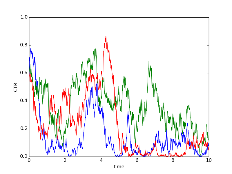
To get a picture of what this model means, I've plotted three possible trajectories below. All of them start out at CTR=60%, but change over time according to the random walk model.

random walk

Before continuing I perform a simple variable transformation - I define $@ Z_t = 2 X_t-1$@. Jacobi diffusion for $@ Z_t $@ takes the form:

$$ d Z_t = - \theta \left(Z_t - \frac{b-a}{a+b+2} \right) dt + \sqrt{ \frac{2 \theta}{a+b+2} (1-Z_t^2) } dW_t $$

Then let us define $@f(z,t)$@, which represents the probability density of $@ Z_t $@ given a specific time. To get from the equation of the random walk to an equation for $@ f(z,t) $@, I use a technique from mathematics called Ito's Lemma. The result of applying Ito's Lemma to the random walk model yields a Partial Differential Equation for $@ f(z,t) $@:

$$ \frac{\partial f(z,t) }{\partial t} = \frac{\partial }{\partial z} \theta \left[ z - \frac{b-a}{a+b+2} \right] f(z,t) + \frac{\partial^2 }{\partial z ^2} \sqrt{\frac{ \theta }{ 2(a+b+2) }} \sqrt{1-z^2} f(z,t)$$

This equation is also called the Fokker-Planck equation.

I'm not actually going to describe how to solve the Fokker-Planck equation right now (hint: Sturm-Liouville theory, noting that it's a Jacobi Equation - see section 2.4 of this paper). I may do that in a future blog post. Instead I'm simply going to discuss the important components of the solution.

The underlying function $@f(z,t)$@ is the probability distribution representing the uncertainty at time $@t$@. I.e., if I plug in a specific value of $@ t$@ - say $@ t=2 $@, then $@ f(z,2) = P(Z=z | t=2)$@ is the probability density for the variable $@Z_2$@.

The Partial Differential Equation describing $@ f(z,t) $@ is an initial value problem. This means that given knowledge of $@ f(z,0) $@, you can compute $@ f(z, t > 0) $@. In python terms, one could represent it as follows:

# An array representing f(z,0)
f0 = [0.0, 0.0, 0.001, ..., 0.25, ..., 0.0]
# f0 represents [f0(-1), f0(-1+dz), f0(2dz), ..., f0(Mdz)],
# where M dz = 2

dt = 0.01 # or some small value
tmax = 5 # the final time I am interested in
f = f0

def right_hand_side(g):
    # code to compute partial derivatives of g,
    # multiply by sqrt(1-z*z), etc
    # Basically compute the right hand side of
    # the Fokker Planck equation
    ...

for i in range(int(tmax/dt)):
    f = f + right_hand_side(f)*dt

    # at this iteration, f represents f(z, i*dt)
    # it can be plotted as necessary

The input f0(z) is a function representing the probability distribution of the CTR at time t0 and the output result(x) is a function representing the probability distribution of the CTR at time t.

I actually use a different method of solution (spectral methods), this conceptually simpler method is simply used here for explanatory purposes.

Behavior of the Fokker-Planck solution

One important fact to understand is that $@ f(z,t) $@ is dissipative, which means that we lose information with time. If we start with a very sharp probability distribution, after some time that solution will spread out and our uncertainty will increase. One way to understand this is to plot $@ f(z,t) $@ at several different values of $@ t $@. At $@ t=0 $@, $@ f(z, 0) $@ is very localized - it's nearly zero except between x=0.2 and x=0.45. Over time, this distribution spreads out.

dissipative solution

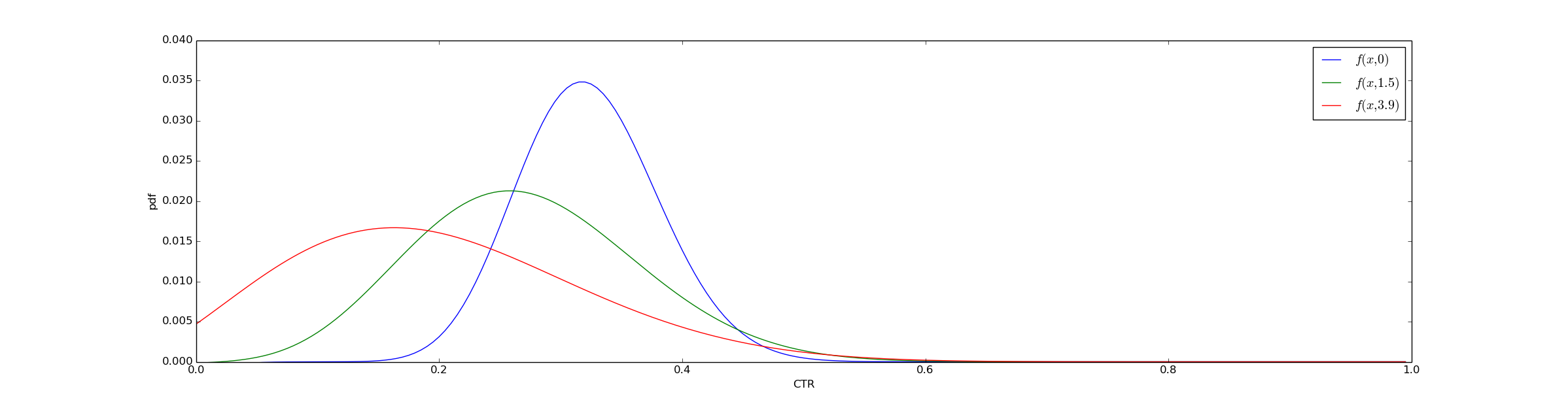
To translate the math to python again, you can think of this graph as being generated simply via the code:

for i in range(int(tmax/dt)):
    f = f + right_hand_side(f)*dt

    if (t*dt == 0):
    plot(x, f, label='$f(x,0)')
    if (t*dt == 1.5):
    plot(x, f, label='$f(x,1.5)')
    if (t*dt == 3.9):
    plot(x, f, label='$f(x,3.9)')

Another way to visualize this is with a heatmap. At time=0 (the left side of the heatmap), the solution is concentrated, while at time=4 the solution is spread out. I've superimposed 3 examples of a random walk on the density plot, which are represented by the black lines. As time increases, the black lines roughly correspond to the locations of high probability.

dissipative solution

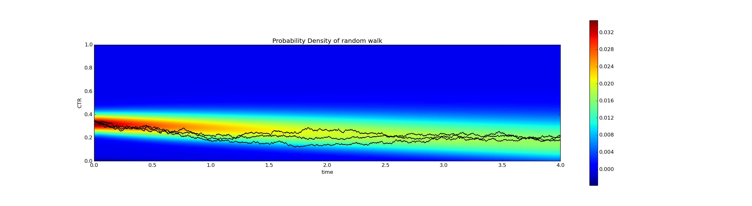
Code to generate this is available here.

Stationary Distribution

An important fact to recognize is that this model has a stationary solution:

$$ q_0(x) = \textrm{const}(1-x)^a x^b$$

This is a beta distribution with parameters $@(a,b)$@. This means that if our prior modelled by $@q_0(x)$@, it will remain $@q_0(x)$@ forever. This means that no matter what information we have now about the CTR, eventually the only information we will have is that it is distributed according to $@ q_0(x) $@.

This stationary solution gives a great method of checking whether I screwed up my calculations somewhere (e.g., flipping a minus sign, losing a factor of 2). We can start with our random walk model, and use a numerical integrator to solve it:

gaussian_var = norm()
def dW(dt):
    return norm.rvs() / sqrt(dt)

def random_walk(z0, tmax, dt, times = None):
    def rhs(z,t):
        return -theta*(z-(a-b)/(a+b+2)) + sqrt(2*theta*(1-z*z)/(a+b+2))*dW(dt)
    if (times is None):
        times = arange(0,tmax,dt)
    z = zeros(shape=times.shape, dtype=float)
    z[0] = z0
    for i in range(1,z.shape[0]):
        z[i] = z[i-1] + rhs(z[i-1], times[i])*dt
        if abs(z[i]) > 1:
            z[i] = z[i] / abs(z[i])
    return (times, z)

Then we can run the simulation many times, and save the value z at the end of the simulation. If we choose tmax to be sufficiently large, the distribution of these values should approach the stationary solution of the Partial Differential Equation. So if we fit a beta distribution to that data, it should agree with the theoretical result. Pseudocode to do this:

end_values = zeros(shape=(N,), dtype=float)
for i in range(N):
    t, y = random_walk(0.25, tmax, 0.01, t)
    end_values[i] = y[-1]

end_values_as_probability = (end_values+1)/2
best_fit = beta.fit(end_values_as_probability, floc=0, fscale=1)
# Result should be approximately (1, 4, 0, 1) - first two params represent beta dist params, second two are floc and fscale

I did this, and plotted the result below. The first plot is a histogram of the terminal positions of z, while the second is the best fit and theoretical distributions:

long_term_random_walk_result

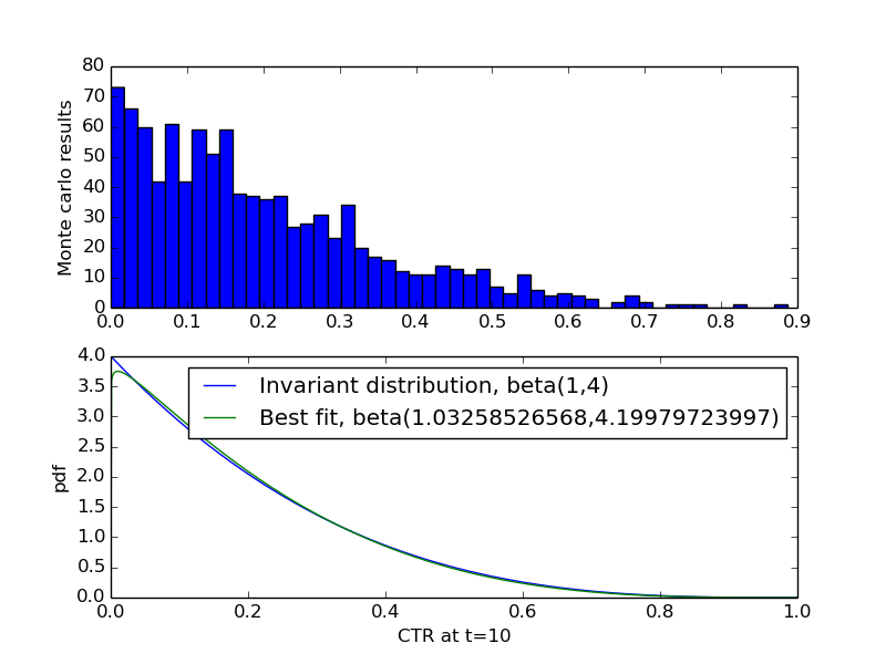
The result is imperfect due to sampling, but it appears more or less correct. To be precise, it's correct the second time I tried - the first version of my math did make a stupid calculation mistake (lost a factor of 2 somewhere), which this method revealed.

Computing a posterior on $@x$@

To compute the posterior distribution for the CTR, we do the following. Suppose at time $@ t=0 $@ we have some distribution on $@ z $@, call it $@ p_0(z) $@. For example, suppose at exactly $@ t=0 $@, we showed the call to action to 40 people resulting in 14 clicks. We then computed a posterior $@ p_0(z) $@ based on the techniques in this blog post.

Now suppose we've waited until $@ t = 0.2 $@. We want to know the posterior now, which is not the same as the posterior at $@ t=0 $@. So we do the following. We solve the Fokker-Planck equation for $@ f(z,0.2) $@ with $@ f(z,0) = p_0(z) $@, and this represents our new posterior.

Imagine it is now $@ t=1.0 $@. Suppose that at this time we display the given call to action to some specific user. If a conversion occurs, we must update our posterior based on this new information:

$$ \textrm{posterior}(x) = \frac{ x f(x, 1.0) } { \int x f(x, 1.0) dx } $$

Conversely, if no conversion occurred, the posterior would be:

$$ \textrm{posterior}(x) = \frac{ (1-x) f(x, 1.0) } { \int (1-x) f(x, 1.0) dx } $$

Now the question arises - what information do we have at time $@ t=1.1 $@? At time $@ t = 1.0 $@, we know that the CTR is distributed according to $@ \textrm{posterior}(x) $@. So to figure out what we know about the distribution of the CTR at $@ t=1.1 $@, we solve the Partial Differential Equation again. But this time, we take $@ f(x, 1.0) = \textrm{posterior}(x) $@ as our initial condition, and solve the equation for an additional $@ 0.1 $@ seconds into the future (from $@ t=1.0 $@ to $@t=1.1$@).

To illustrate this process, I ran the following simulation. I first chose a "true" CTR based on the random walk simulation. Then I solved the Fokker-Planck equation from t=0 to t=1. At time t=1, I drew 30 samples from the true CTR, as follows:

nsamples = 30
r = rnd.rvs(nsamples)
success = (r < true_ctr).sum()
fails = 30 - success

I then performed a Bayesian update on $@ f(x, t) $@ and continued the simulation. In pythonic code, the Bayesian update consisted of:

def bayesian_update(success, fails, f_before_update):
    # At the start, f_before_update is an array, something like this: [ 0.0, 0.01, 0.04, ... ]

    x = [ 0.0, 0.01, ..., 0.99, 1.0]
    f_after_update = f_before_update.copy()
    for i in range(success):
        f_after_update *= x
    for i in range(fails):
        f_after_update *= (1-x)

    #Normalization to bring f back to being a probability distribution
    f_after_update /= f_after_update.sum()
    return f_after_update

I repeated the process of drawing samples and updating the evidence at t=2 and t=3. The result is plotted below:

Bayesian Estimate of CTR

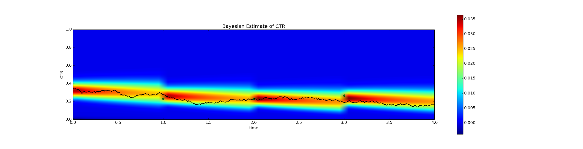
There is a lot happening in this graph. The black line represents the true click through rate. The only reason we can actually graph this is because this is a simulation. In real life the black line would be unobservable.

The green dots represent the empirical click through rate at the relevant time - i.e., the height of the green dot at t=1 represents success / fails. This of course is measurable in real life.

Finally, the color of the graph represents the Bayesian probability density

Here is actual runnable code (rather than illustrative pseudocode) which handles the bayesian update. It's harder to understand, but on the plus side it actually works.

The effect of flukes

The answer is of course yes. If by some improbable fluke, the true conversion rate is 20%, but you observe empirically that it is 100%, your estimates will be off. This is unavoidable.

But when you observe flukes caused by a small sample size, these will not affect your estimates as much as you might expect. Consider the following simulation, identical to the previous one, except that I've reduced the sample size, i.e. nsamples = 10. I ran a simulation where at t=2 an improbable fluke occurs - the empirical conversion rate was 60% (6/10) even though the actual conversion rate was about 25%. Although unlikely, this will occur occasionally. The result is plotted below.

Bayesian Estimate of CTR

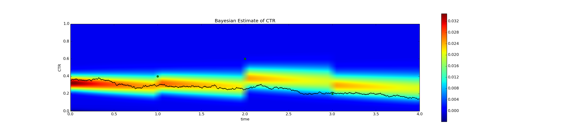
The Bayesian estimator is certainly an overestimate at t=2.1. But the estimated conversion rate has not increased 60% - according to the posterior, the probability that CTR >= 60% is still negligably low.

Isn't this just Black Scholes?

Readers familiar with derivative pricing are probably asking themselves - is this guy an ex-trader? (Answer: Yes.) There is a strong similarity between the techniques of mathematical finance and what I did here. For example, the Black-Scholes random-walk is:

$$ dS_t = \mu S_t + \sigma dW_t $$

where $@ S_t $@ represents the price of a security at time $@ t $@. Although a little different, the hard parts of this equation are very similar to the equation of the random walk of a CTR. Mathematically I used all the same techniques as in derivative pricing - Ito's Lemma and partial differential equations.

But it's important to note that while the math is similar, what I'm doing here is fundamentally different from derivative pricing. Derivative pricing takes place in the Q-world of risk-neutral probabilities, which fundamentally do not represent beliefs about what will happen in the future. A quant trader has certain knowledge of the future - at the expiration date, the value of an option is known precisely. Given this certain knowledge of the future, the quant attempts to make "predictions" about the present, namely the true value of an option today. If the "true value" of the option differs from the market value, the quant can make money.

In contrast, the calculation I perform here takes place in the P-world and represent beliefs about the future. I have uncertain knowledge about the present, namely the empirical click through rate (not to be confused with the true click through rate), and my goal is to predict the click through rate in the future. Further, the concept of a Bayesian update based on new evidence is entirely absent in derivative pricing, at least as far as I'm aware.

Conclusion

Conversion rates vary with time. Unless you have enough data to accurately measure conversion rates every day, this poses a big problem for you. Fortunately, Bayesian Statistics provides a fairly straightforward (albeit somewhat computationally tricky) method of tracking them. In a future blog post, I'll explain how to use this method not only to predict what the conversion rate will be in the future, but to actually build a bandit algorithm to track a changing conversion rate.

The paper A stochastic diffusion process for the Dirichlet Equation does something similar, but for the Dirichlet Distribution rather than the Beta Distribution. Could come in handy if you need to bucket into more than 2 categories (e.g., [ NoConvert, ConvertToX, ConvertToY]).

Also relevant is The Pearson diffusions: A class of statistically tractable diffusion processes and On Properties of Analytically Solvable Families of Local Volatility Diffusion Models.

John Boyd's book Chebyshev and Fourier Spectral Methods provides an excellent (and pretty cheap, under $30) introduction to solving PDEs like the one here.

For anyone interested in mathematical finance in addition to the math I describe here, the book Quantitative Finance by Wilmott is a good introduction. It introduces Partial Differential Equations, Black Scholes and Monte Carlo methods as well as a lot of the terminology of finance.

I imagine there is more out there in the literature than this. But I've never been much good at literature searches, and most of it is probably behind an academic paywall anyway. But if anyone has pointers, I'd love to see them.