I'm currently dating two lovely women, Svetlana and Elise. Unfortunately continuing to date both of them is unsustainable so I must choose one.

In order to make such a choice, I wish to construct a ranking function - a function which takes as input the characteristics of a woman and returns as output a single number. This ranking function is meant to approximate my utility function - a higher number means that by making this choice I will be happier. If the ranking closely approximates utility, then I can use the ranking function as an effective decisionmaking tool.
In concrete terms, I want to build a function $@ f : \textrm{Women} \rightarrow \mathbb{R} $@ which approximately predicts my happiness. If $@ f(\textrm{Svetlana}) > f(\textrm{Elise}) $@ I will choose Svetlana, and vice versa if the reverse inequality holds.
One of the simplest procedures for building a ranking function dates back to 1772, and was described by Benjamin Franklin:
...my Way is, to divide half a Sheet of Paper by a Line into two Columns, writing over the one Pro, and over the other Con. Then...I put down under the different Heads short Hints of the different Motives...I find at length where the Ballance lies...I come to a Determination accordingly.
The mathematical name for this technique is unit weighted regression, and the more commonplace name for it is a Pro/Con list.
I present the method in a slightly different format - in each column a different choice is listed. Each row represents a characteristic, all of which are pros. A con is transformed into a pro by negation - rather than treating "Fat" as a con, I treat "Not Fat" as a pro. If one of the choices possesses the characteristic under discussion, a +1 is assigned to the relevant row/column, otherwise 0 is assigned:
| Characteristic | Elise | Svetlana |
|---|---|---|
| Smart | 0 | +1 |
| Great Legs | +1 | +1 |
| Black | +1 | 0 |
| Rational | 0 | 0 |
| Exciting | +1 | 0 |
| Not Fat | +1 | +1 |
| Lets me work | 0 | 0 |
Unit-weighted regression consists of taking the values in each column and adding them up. Each value is either zero or one. The net result is that $@ f(\textrm{Elise}) = 4 $@ and $@ f(\textrm{Svetlana}) = 3 $@. Elise it is!
Pro/Con lists are easy
A pro/con list is one of the simplest ranking algorithms you can construct. The mathematical sophistication required is grade school arithmetic and it's so easy to program that even a RoR hipster could do it. As a result, you should not hesitate to implement a pro/con list for decision processes.
The key factor in the success of unit-weighted regression is feature selection. The rule of thumb here is very simple - choose features which you have good reason to believe are strongly predictive of the quantity you wish to rank. Such features can usually be determined without a lot of data - typically a combination of expert opinion and easy correlations are sufficient. For example, I do not need a large amount of data to determine that I consider "not fat" to be a positive predictor of my happiness with a woman.
Conversely, if the predictiveness of a feature is not clear, it should not be used.
Why not use machine learning (TM)?
Anyone who read one of the many good books on machine learning can probably name several fancy machine learning techniques - neural networks, decision trees, etc. And they are probably asking why I would ever use unit-weighted regression, as opposed to one of these techniques? Why not use linear regression, rather than forcing all the coefficients to be +1?
I'll be concrete, and consider the case of linear regression in particular. Linear regression is a lot like a pro/con list, except that the weight of each feature is allowed to vary. In mathematical terms, we represent each possible choice as a binary vector - for example:
Then the predictor function uses a set of weights which can take on values other than $@ +1 $@:
The individual weights $@ f_i $@ represent how important each variable is. For example, "Smart" might receive a weight of +3.3, "Not fat" a weight of +3.1 and "Black" a weight of +0.9.
The weights can be determined with a reasonable degree of accuracy by taking past data and choosing the weights which minimize the difference between the "true" value and the approximate value - this is what least squares does.
The difficulty with using a fancier learning tool is that it only works when you have sufficient data. To robustly fit a linear model, you'll need tens to hundreds of data points per feature. If you have too few data points, you run into a real danger of overfitting - building a model which accurately memorizes the past, but fails to predict the future. You can even run into this problem if you have lots of data points, but those data points don't represent all the features in question.
It also requires more programming sophistication to build, and more mathematical sophistication to recognize when you are running into trouble.
For the rest of this post I'll be comparing a Pro/Con list to Linear Regression, since this will make the theoretical comparison tractable and keep the explanation simple. Let me emphasize that I'm not pushing a pro/con list as a solution to all the ranking problems - I'm just pushing it as a nice simple starting point.
A Pro/Con list is 75% as good as linear regression
This is where things get interesting. It turns out that Pro/Con list is at least 75% as good as a linear regression model.
Suppose we've done linear regression and found linear regression coefficients $@ \vec{h} $@. Suppose instead of using the vector $@ \vec{h} $@, we instead used the vector of unit weights, $@ \vec{u} = [ 1/N, 1/N, \ldots, 1/N] $@. Here $@ N $@ is the number of features in the model.
An error is made whenever the pro/con list and linear regression rank two vectors differently - i.e., linear regression says "choose Elise" while the pro/con list says "choose Svetlana". The error rate of the pro/con list is the probability of making an error given two random feature vectors $@ \vec{x} $@ and $@ \vec{y} $@, i.e.:
It turns out that if you average it out over all vectors $@ \vec{h} $@, the error rate is bounded by 1/4. There are of course vectors $@ \vec{h} $@ for which the error rate is higher, and others for which it is lower. But on average, the error rate is bounded by 1/4.
In this sense, the pro/con list is 75% as good as linear regression.
We can confirm this fact by computer simulation - generating a random ensemble of vectors $@ \vec{h} $@, and then measuring how accurately unit-weighted regression agrees with it. The result:
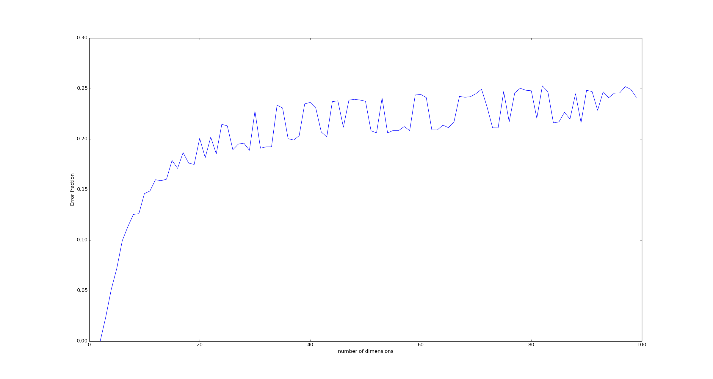
More concretely, I computed this graph via the following procedure. For every dimension N, I created a large number of vectors $@ \vec{h} $@ by drawing them from the uniform Dirichlet Distribution. This means that the vectors $@ \vec{h} $@ were chosen so that:
and
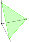
In 3 dimensions, this means that $@ \vec{h} $@ lives on the green surface in this figure:
Then I generated a set of vectors $@ \vec{x}, \vec{y} $@ by choosing each component to be 0 or 1 with a probability of 50% each.
Mathematical results
I don't know how to prove how closely a Pro/Con list approximates linear regression for binary feature vectors. However, if we assume that the feature vectors $@ \vec{x} $@ and $@ \vec{y} $@ are normally distributed instead, I can prove the following theorem:
Theorem: Suppose $@ \vec{h} $@ is drawn from a uniform Dirichlet distribution and $@ \vec{x}, \vec{y} $@ have components which are independent identical normally distributed variables. Then:
This means that averaged over all vectors $@ \vec{h} $@, the error rate is bounded by 1/4. There are of course individual vectors $@ \vec{h} $@ with a higher or lower error rate, but the typical error rate is 1/4.
Unfortunately I don't know how to prove this is true for Bernoulli (binary) vectors \(@ \vec{x}, \vec{y}\)@. Any suggestions would be appreciated.
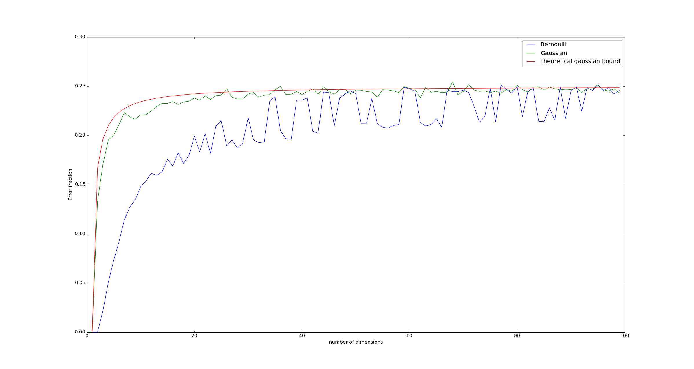
If we run a Monte Carlo simulation, we can see that this theorem appears roughly correct:
Code to produce the graph is available on github.
In fact, the graph suggests the bound above is close to being exact. The theorem is proved in the appendix.
Appendix: Proof of the error bound
Let us consider a very simple, 3-dimensional example to build some intuition. In this example, $@ \vec{h} = [ 0.9, 0.05, 0.05] $@ - a bit of an extreme case, but reasonable. In this example, what sorts of vectors $@ \vec{x}, \vec{y} $@ will result in unit-weighted regression disagreeing with the true ranking? Here is one example:
In this case, $@ \vec{h} \cdot (\vec{x} - \vec{y}) = 0.8 $@ wereas $@ \vec{u} \cdot (\vec{x} - \vec{y}) = -1/3 $@.
Intuitively, what is happening here is that the vector $@ \vec{x} $@ is pointing nearly in the same direction as $@ \vec{h} $@, while the vector $@ \vec{y} $@ is nearly perpendicular to it.
Normally distributed feature vectors
Suppose for simplicity that the feature vectors $@ \vec{x}, \vec{y} $@ satisfy $@ \vec{x}_i \sim N(0,2^{-1/2}) $@. Define $@ \vec{d} = \vec{x} - \vec{y} $@, and note that $@ \vec{d}_i \sim N(0,1) $@. This is an unrealistic assumption, but one which is mathematically tractable. We want to compute the probability:
For simplicity, we will attempt to compute the latter quantity.
How accurately does $@ \vec{u} $@ approximate $@ \vec{h} $@?
Define $@ \vec{h} = \vec{u} + \vec{p} $@ where $@ \vec{p} \cdot \vec{u} = 0 $@. Then:
Note that $@ \vec{d} $@ is generated by a multivariate normal distribution, with covariance matrix equal to the identity. As a result:
where $@ N $@ is the dimension of the problem. Similarly:
Due to the orthogonality of $@ \vec{u} $@ and $@ \vec{p} $@, the quantities $@ \vec{u} \cdot \vec{d} $@ and $@ \vec{p} \cdot \vec{d} $@ are independent.
Note: Obtaining this statistical independence is why we needed to assume the feature vectors were normal - showing statistical independence in the case of binary vectors is harder. A potentially easier test case than binary vectors might be random vectors chosen uniformly from the unit ball in \(@ l^\infty $@, aka vectors for which $@ \max_i |\vec{x}_i| < 1\)@.
We've now reduced the problem to simple calculus. Define $@ \sigma_u^2 = N^{-1} $@ and $@ \sigma_p^2 = \sum \vec{p}_i^2 $@. Let $@ v = \vec{u} \cdot \vec{d} $@ and $@ w = \vec{p} \cdot \vec{d} $@. Then:
Changing variables to $@ v = r \sigma_u \cos(\theta) $@, $@ w = r \sigma_p \sin(\theta) $@. Then:
Here $@ \theta_0 = \textrm{arccot}(\sigma_u/\sigma_p) $@, so:
Worse case analysis
The worst case to consider is when \(@ \vec{h}\)@ is one of the corners of the unit simplex - e.g. $@ \vec{h} = [1,0,\ldots,0] $@. In this case:
So $@ \sigma_p = \sqrt{(N-1)/N} $@ while $@ \sigma_u = 1/\sqrt{N} $@, and $@ \textrm{arccot}( -1/\sqrt{N-1} ) \rightarrow \pi $@ as $@ N \rightarrow \infty $@. This implies:
This means that in the worst case, unit-weighted regression is no better than chance.
Average case analysis
Let us now consider the average case over all vectors $@ \vec{h} $@. To handle this case, we must impose a probability distribution on such vectors. The natural distribution to consider is the uniform distribution on the unit-simplex, which is equivalent to a Dirichlet distribution with $@ \alpha_1 = \alpha_2 = \ldots = \alpha_N = 1 $@.
So what we want to compute is:
This can be bounded above as follows, noting that $@ \sigma_p = \sqrt{| \vec{h} - \vec{u}|^2} $@:
The inequality follows from Jensen's Inequality since $@ z \mapsto \arctan(\sqrt{N} \sqrt{z}) $@ is a concave function.
For large $@ N $@ this quantity approaches $@ \arctan(1) / 2 \pi = (\pi/4) / (2\pi) = 1/8 $@.
Thus, we have shown that the average error-rate of unit-weighted regression is bounded above by $@ 1/4 $@. It also shows that treating feature vectors as Gaussian rather than Boolean vectors appears to be a reasonable approximation to the problem - if anything it introduces extra error.
Note: I believe that the reason the Bernoulli feature vectors appear to have lower error than the Gaussian feature vectors for small N appears to be caused by the fact that for small N, there is a significant possibility that a feature vector might be 0 in the relevant components. The net result of this is that $@ \vec{h} \cdot (\vec{x} - \vec{y}) = 0 $@ fairly often, meaning that many vectors have equal rank. This effect becomes improbable as more features are introduced.
Frequently Asked Questions
All the pre-readers I shared this with had two major but tangential questions which are worth answering once and for all.
First, Olga Kurylenko and Oluchi Onweagba.
Second, I didn't waste time with gimp. Imagemagick was more than sufficient:
# -resize x594 will shrink height to 594, preserve aspect ratio
$ convert olga-kurylenko-too-big.jpg -resize 'x594' olga-kurylenko.jpg;
# -tile x1 means tile the images with 1 row, however many columns are needed
$ montage -mode concatenate -tile x1 olga-kurylenko.jpg oluchi-onweagba.jpg composite.jpg