Great news! A murder victim has been found. No slow news day today! The story is already written, now a title needs to be selected. The clever reporter who wrote the story has come up with two potential titles - "Murder victim found in adult entertainment venue" and "Headless Body found in Topless Bar". (The latter title is one I've shamelessly stolen from the NY Daily News.) Once upon a time, deciding which title to run was a matter for a news editor to decide. Those days are now over - the geeks now rule the earth. Title selection is now primarily an algorithmic problem, not an editorial one.
One common approach is to display both potential versions of the title on the homepage or news feed, and measure the Click Through Rate (CTR) of each version of the title. At some point, when the measured CTR for one title exceeds that of the other title, you'll switch to the one with the highest for all users. Algorithms for solving this problem are called bandit algorithms.
In this blog post I'll describe one of my favorite bandit algorithms, the Bayesian Bandit, and show why it is an excellent method to use for problems which give us more information than typical bandit algorithms.
Unless you are already familiar with Bayesian statistics and beta distributions, I strongly recommend reading the previous blog post. That post provides much introductory material, and I'll depend on it heavily.
The problem to be solved, and the underlying model
Ultimately the problem we want to solve is the following. Consider an article being published on a website. The author or editor has come up with several possible titles - "Murder victim found in adult entertainment venue", "Headless Body found in Topless Bar", etc. We want to choose the title with the best click through rate (CTR). Let us represent each CTR by \(@\theta_i\)@ - i.e., \(@\theta_i\)@ is the true probability that an individual user will click on the i-th title. As a simplifying assumption, we assume that these rates \(@\theta_i\)@ do not change over time. It is important to note that we don't actually know what \(@\theta_i\)@ is - if we did, we could simply choose \(@i\)@ for which \(@\theta_i\)@ was largest and move on.
The goal of the bandit algorithm is to do the following. To begin with, it should display all possible titles to a random selection of users, and measure which titles are clicked on more frequently. Over time, it will use these observations to infer which articles have the higher CTR. Then, once the estimation of the CTR becomes more precise, it will preferentially display articles with the higher CTR.
The Bayesian Approach
In the model described above, we have \(@N\)@ possible story titles, each of which has a click through rate \(@\theta_i\)@. Unfortunately we do not know what \(@\theta_i\)@ is. As the astute reader can guess from the title, we are following a Bayesian approach, so we will construct a probability distribution which represents our belief about what the actual value of \(@\theta_i\)@ is.
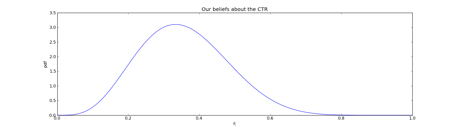
In the figure above, we believe that \(@\theta_i\)@ is somewhere between 0.1 and 0.7, with values of 0.3-0.4 being considerably more likely than values of 0.1-0.2 or 0.6-0.7. For those who forgot STATS 101, the area under this curve between the points a and b is the probability thta \(@\theta_i\)@ lies between a and b. I.e.:
The basic idea behind Bayesian methods is to update our beliefs based on evidence. As we gather more data by showing different titles to other users and observing click throughs, we can incrementally narrow the width of the probability distribution.
As in all Bayesian inference, we need to choose a prior. The prior is something we believe to be true before we have any evidence - i.e., before we have shown the title to any visitors. This is just a starting point - after enough evidence is gathered, our prior will play a very minimal role in what we actually believe. Choosing a good prior is important both for mathematical simplicity, and because if your prior is accurate, you don't need as much evidence to get the correct answer.
I'll follow the approach I described in a previous blog post, and I'll use a beta distribution as the prior:
The parameters \(@\alpha_i, \beta_i > 1\)@ are the prior parameters. One reasonable choice is \(@\alpha_i=\beta_i=1\)@, which amounts to the uniform distribution on \(@[0,1]\)@. What this means is that we are assuming that all possible values of \(@\theta_i\)@ are equally likely. Depending on the circumstances (which I'll explain shortly), we might want to choose other possible values.
Updating our beliefs
Now we address the question of using evidence.
After showing title \(@i\)@ to \(@n_i\)@ visitors, we have observed that \(@s_i\)@ of them have actually clicked on the title. We now want to compute the posterior distribution, which is to say the distribution that represents our beliefs after we have evidence.
I did a little bit of algebra previously, in which I showed that if the prior is \(@f_{\alpha_i, \beta_i}(\theta_i)\)@, then the posterior distribution is:
The key idea here is that to update our probability distribution describing \(@\theta_i\)@, we need only update the parameters of our beta distribution.
So what does this mean in practice? As we run more experiments, our probability distribution on where \(@\theta_i\)@ lives becomes sharper:
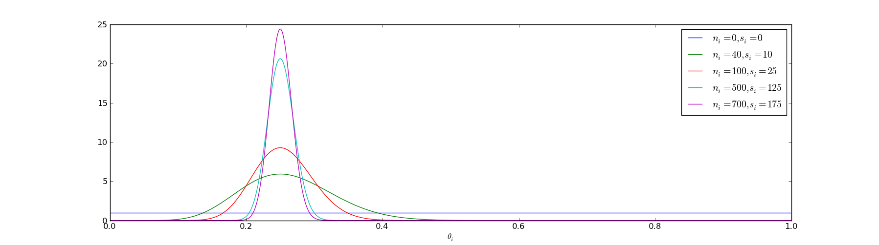
Before we run any experiments, \(@\theta_i\)@ could be anything (as represented by the blue line). Once we have run 700 experiments, yielding 175 click throughs, we are reasonably confident that \(@\theta_i\)@ lives roughly between 0.2 and 0.3.
What we've done so far is figured out how to estimate what our click through rates actually are based on empirical evidence. But that doesn't actually give us a method of optimizing them yet.
Optimizing click throughs
Now that we have a method of representing our beliefs about CTRs, it is useful to construct an algorithm to identify the best ones. There are many popular choices - I've written about the UCB Algorithm before, and I consider it a good choice.
But my new favorite method is a Monte Carlo method which I'll describe now.
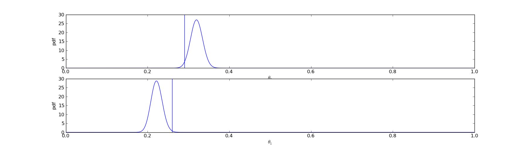
The ultimate goal of the bandit algorithm is to display to the user whichever title has the highest CTR. One method of estimating the CTRs of the articles is to sample the posterior distribution. I.e., suppose we have two possible titles, from which we have drawn \(@n_0=200, s_0=64\)@ and \(@n_1=180, n_2=40\)@. Then one possible set of samples we might observe is this:
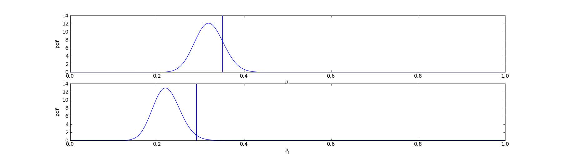
For title 0, our sample of \(@\theta_0\)@ has worked out to be 0.35, while our sample of \(@\theta_1\)@ is only 0.28. Since \(@\theta_0 = 0.35 > \theta_1 = 0.28\)@, we will display title 0 to the user.
However, there was no guarantee that things worked out this way. It was possible, although less likely, that \(@\theta_1\)@ could come out larger than \(@\theta_0\)@:
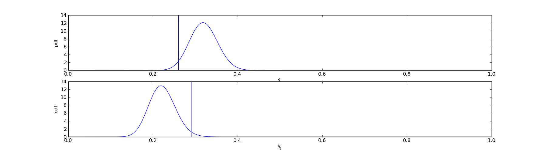
In this case, we would have displayed title 1 to the user rather than title 0.
The net result is that for overlapping probability distributions, we will display the title with the larger expected CTR the majority of the time. But occasionally, we will draw from the other distributions simply because it is within the realm of possibility that they are greater.
As we gather more data our probability distributions will become narrower and a clear winner will become apparent. When this occurs, we will almost surely choose the winner:
In python, the algorithm looks like this:
The results of this algorithm are exactly what any good bandit algorithm should do. I ran the following simulation, giving the beta bandit two titles - title 0 had a CTR of 0.25, title 1 had a CTR of 0.35. To start with, both titles were displayed to the user with roughly equal probability. Over time, evidence accumulated that title 1 was considerably better than title 0. At this point the algorithm switched to displaying primarily title 1, and the overall CTR of the experiment converged to 0.35 (the optimal CTR).
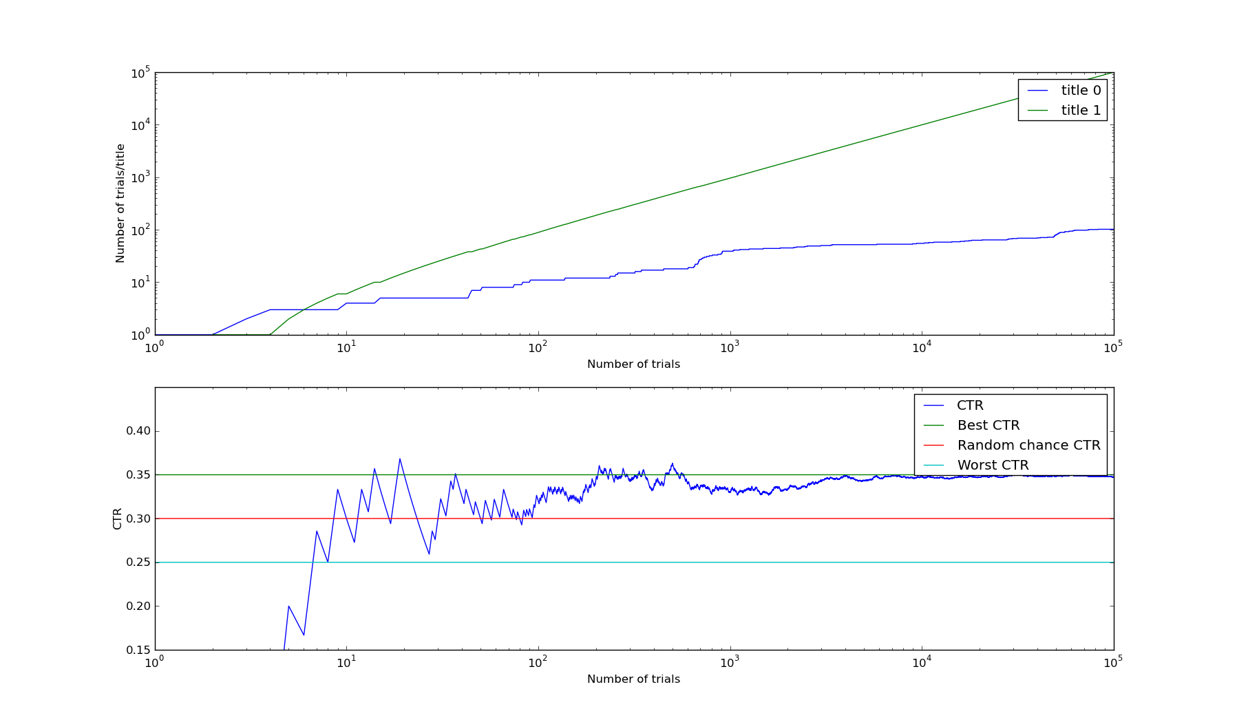
Source code to generate this graph is available here. This method is called Thompson Sampling and is a a fairly popular method in Bayesian AI techniques. For the remainder of this post, I'll call this method the Bayesian Bandit.
Incorporating common sense
Anyone with common sense is now scoffing at the geekiness embodied in this post. Even before using statistics, it was fairly obvious that "Headless Body found in Topless Bar" was going to beat "Murder victim found in adult entertainment venue". The former just sounds catchier and any good editor would run with it.
The wonderful thing about Bayesian methods is that we can modify them to take into account our prior knowledge. Suppose we believe editors intuition is a real thing - can we quantify it? Certainly. We can do this with a fairly simple experiment. We require editors to rate a collection of titles as "catchy" or "not catchy", run them on the site, and then measure the CTR of the "catchy" and "not catchy" samples. Suppose we did such an experiment, and observed the following aggregate results:
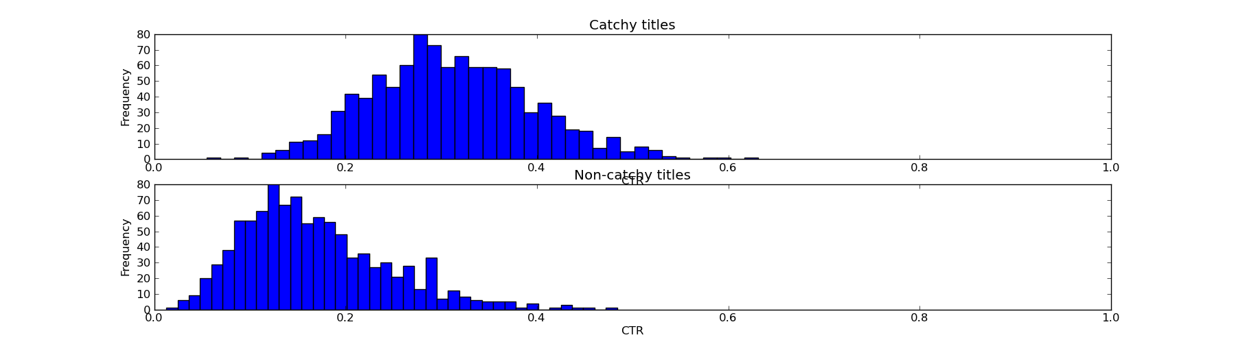
This isn't a solid win for the editor - some catchy titles have low CTRs, and some boring titles have good CTRs. But nevertheless, it's better for a story to have catchy title than not.
What we want to do is incorporate this information into our bandit algorithm. The beauty of a Bayesian method is that it gives you a clear and meaningful place to plug this information in, namely the prior. In contrast, for many other methods (e.g., UCB) it's somewhat difficult to do this - there is no obvious parameter to tune as a result of our prior empirical data.
The first step is to fit a theoretical distribution to the empirical data. Due to the fact that I chose the "empirical" (i.e., made up) data to be very nice, a beta distribution fits well [1] - specifically beta distributions with \(@(\alpha_0, \beta_0) = (9,20)\)@ and \(@(\alpha_1, \beta_1) = (4,20)\)@.
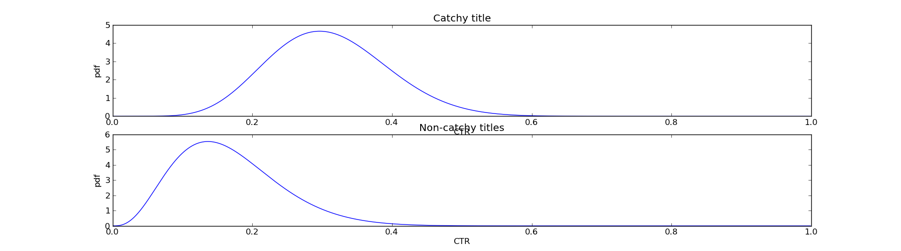
Then the only modification needed to the algorithm is to plug these variables into the prior:
Everything else remains unchanged. In terms of modifications to source code, this is only a very small change to the previous code - an implementation can be found here.
Empirics of including priors
To measure the benefits of incorporating priors into the Bayesian bandit, I ran some numerical experiments, the source code of which is available in this github gist. The methodology was the following.
To compare the Bayesian bandit with priors to that without, I drew a pair \(@(\theta_0, \theta_1)\)@ from the prior distribution given above. For each pair, I then ran the Bayes Bandit with and without priors for this pair theta, for \(@k\)@ trials. This is modelling the scenario that we have \(@k\)@ page views on our homepage, and we can only leave a story on the homepage for 1 day.
I then repeated the experiment for 1000 different possible days, or equivalently for 1000 different pairs of \(@(\theta_0, \theta_1)\)@. I then computed the average gain per page view over all trials and all days.
The result is the following. If we get 50 page views/day (i.e., the Bayes Bandit has very little data to use), the prior gives us a big gain. Without prior knowledge, the Bandit achieved a gain of 0.3749 on average, whereas the bandit with prior knowledge achieved a gain of 0.4274. If we run 150 experiments, the Bayes Bandit improves significantly - it achieves a gain of 0.40. If we run 300 experiments, the Bayes Bandit improves to 0.4146, while the bandit with priors improves to 0.4296. If we get 1000 page views/day, the Bayes Bandit improves to 0.4211, while the bandit with priors gains 0.4249.
The net result is the following - incorporating priors into the Bayes Bandit is an excellent way to improve your results when you don't have a large number data points to use to train the bandit. If you have a lot of data points, you don't need strong priors (but they still help a little).
Conclusion
Bandit algorithms are a great way of optimizing many factors of your website. There are many good options - I've written about UCB before and consider it a great choice. But if you have other information you want to include, consider using the Bayesian Bandit. It's simple to implement, straightforward to use, and very importantly it's also straightforward to extend.
It's also important to note that the theoretical properties of the Bayesian Bandit (namely logarithmic regret) have been proven. So asymptotically, you lose nothing by using it. There are also attempts at constructing a Bayesian UCB algorithm - I don't currently understand it well enough to comment.
I've written other articles related to this post. I have one post comparing bandit algorithms to a/b testing. I also I wrote about measuring a changing conversion rate, which provides an alternate algorithm for computing the posterior distribution if your conversion rate is not constant.
[1] If a single Beta distribution doesn't fit, one can also use a convex combination of Beta distributions. The math works out just as nicely.
P.S. After I published this blog post, this related article was also pointed out to me, as was this online simulation of the Bayesian bandit.