Very often one builds a statistical model in pieces. For example, imagine one has a binary event which may or may not occur - to work with my thematic example, a visitor arrives on a webpage and he may or may not convert. A reasonable question to ask is "if I have 100 visitors, how many of them can I expect to convert?" Assume now that I know the conversion rate lmbda; in this case the maximum likelihood point estimate for the number of conversions is 100*lmbda and the probability distribution of possible events that could occur is binom(100, lmbda) (i.e. a binomial distribution). But what happens if lmbda is not known, but instead a random variable?
In a previous post, I considered the problem of measuring the detection probability of an individual sensor in a sensor network with delays between detection and reporting. My solution to this problem involved assuming that I knew the detection probability as a function between the current time and the time of detection. I.e., I assumed that I knew exactly the cdf r(t) of the delay. When I showed the delayed reactions post to a critic, one of his immediate reaction was to ask how I'd find r(t). My suggestion was then to use a nonparametric Bayesian estimator, the output of which is a probability distribution over the space of possible functions r(t) as opposed to an individual r(t).
In both cases, I made assumptions that certain quantities were known exactly, and then I used those exact numbers to derive a probability distribution on the quantity of interest. But in reality, those quantities are not known exactly - merely probabilistically.
In this blog post I'll show why this is fundamentally not a problem. That's because probability is a monad and this monadic structure allows me to combine various analysis in a natural and obvious way.
Background: I am assuming that the reader of this post has a moderate amount of knowledge of probability theory, and a moderate amount of knowledge of functional programming. I will be assuming that functors (objects with a map method) and monads (objects which also have flatMap or bind or >>= on them) are known to the reader.
Also, for a more mathematical look at this topic, I'm mostly taking this stuff from the papers A Categorical Approach to Probability Theory (by Giry) and A Categorical Foundation for Bayesian Probability (by Culbertson and Surtz). This post is more intended for programmers than mathematicians.
Probability in the language of type theory
In the language of type theory, probability is a type constructor Prob[T]. An object of this type should be interpreted as being a probability distribution over objects of type T, or a probability measure on T. As the simplest possible measure, lets allow T = Boolean. Then an object in Prob[Boolean] can be thought of as being a function f: Boolean => Real where f(true) + f(false) = 1, f(true) >= 0 and f(false >= 0).
In the language of computer science, there are several alternative ways to represent Prob[T]. The first is simply as a function mapping objects to their probabilities:
trait Prob[T] {
  //Here T is a finite object
  def prob(t: T): Real
}

forAll( (p: Prob[T]) => {
  //allT is a sequence of every possible value of T.
  (allT.map(prob.prob).sum == 1.0)
})

forAll( (p: Prob[T], t: T) => {
  require(p.prob(t) >= 0)
})
A second way to represent it is as a sequence of samples:
trait Rand[T] {
  def draw: T
}
In this case one can approximately recover a Prob[T] object:
class ApproxProb[T](rand: Rand[T]) extends Prob[T] {
  //It doesn't really extend Prob[T], but it comes close
  val numAttempts = 1000000

  def prob(t: T) = {
    var numFound = 0
    var i: Int=0
    while (i < numAttempts) {
      if (rand.draw == t) { numFound += 1 } else { }
      i += 1
    }
    return numFound.toDouble / numAttempts.toDouble
  }
}
This sampling representation will not exactly satisfy the laws that Prob[T] does, but it will come close if numAttempts is large enough.
Stochastic analysis
Relating this problem to the examples above, let us consider first the problem of estimate a future number of conversions. Given a conversion rate lmbda and N visitors, we know that the number of conversions is binomially distributed. We can therefore represent our solution to the problem as a function of type (Real, Integer) => Prob[Integer]:
def numConversions(lmbda: Real, N: Integer): Prob[Integer] =
  new Prob[Integer] {
    def prob(t: Integer) = Binomial(lmbda, N).pmf(t)
  }
(Here pmf is the probability mass function of the binomial distribution.)
We could also define this using the sampling representation:
def numConversions(lmbda: Real, n: Integer): Rand[Integer] =
  new Prob[Integer] {
    def draw = Binomial(lmbda, N).draw
  }
In either case, we are building a function of deterministic inputs and getting a function of type Prob[T] as an output.
Probability is a functor
The first observation which is important to make is that probability is a functor. Specificaly, what this means is that if you have an object of type Prob[T], and a function f: T => U, you can get an object of type Prob[U] out from it. Let me start with a motivating example. Let T be the set {a, b, c}. Then define:
val prob = new Prob[T] {
  def prob(t: T) = 1.0/3.0
}
This probability distribution assigns equal weight (1/3 probability) to each element of T. Now let U be the set {x, y}, and f: T => U be the function:
def f(t: T) = t match {
    case a => x
    case b => x
    case c => y
  }
The result of prob.map(f) should be the probability distribution mapping to x with 2/3 probability and to y with 1/3 probability.
The simpler way to define map is in the sampling representation:
object RandFunctor extends Functor[Rand] {
  def map[T, U](p: Rand[T])(f: T => U): Rand[U] = new Rand[U] {
    def draw: U = f(p.draw)
  }
}
When we have maped a Rand[T], we get a new object which provides random samples of type U.
If we apply this definition to our example above, we discover that 2/3 of the time, the outcome of p.draw is either a or b. As a result, 2/3 of the time the outcome of the mapped distribution is x, as desired.
We can also provide a definition in the Prob[T] representation, but it's a bit more complicated:
object ProbFunctor extends Functor[Prob] {
  def map[T, U](p: Prob[T])(f: T => U): Prob[U] = new Prob[U] {
    def prob(u): Real = {
      val inverseImage: List[T] = allT.filter(t => f(t) == u)
      return inverseImage.map(p.prob _).sum()
    }
  }
}
In this case, we can do the calculations by hand. Suppose we compute prob(u=x). Then the value of inverseImage is the set of all T for which f(t) == x, and this happens to be List(a,b). Next we compute inverseImage.map(p.prob _) which works out to be List(1/3, 1/3). Finally we sum that list, resulting in 2/3.
Woot! Both of our representations work out correctly.
Probability as a monad
Lets consider now the following situation. We run an experiment, and measure our conversion rate as described here. The net result is that we form an opinion on the conversion rate:
val conversionRate = new Rand[Real] {
  def draw = BetaDistribution(numConversions + 1, numVisitors - numConversions + 1).draw
}
Given the previous discussion, we now have the following idea - lets take this and map it with our numConversions function above:
val expectedConversions =
  conversionRate.map(lmbda => numConversions(lmbda, 100))
Unfortunately, if we look at the type of expectedConversions, it works out to be Rand[Rand[Int]]. That's not what we wanted - we really wanted a Rand[Int].
So what we need to do is somehow flatten a Prob[Prob[Int]] or a Rand[Rand[Int]] down to a Prob[Int] or Rand[Int].
In the sampling approach, there is one pretty obvious approach. Recall how we defined map on a Rand[T] object - we applied the function to the result of drawing a random number. What if we draw a new sampel? I'll write an implementation of this and suggestively name it bind:
object RandMonad extends Monad[Rand] {
  def bind[T, U](p: Rand[T])(f: T => Rand[U]): Rand[U] = new Rand[U] {
    def draw: U = f(p.draw).draw
  }
}
Clearly the type signature of this matches. It also makes intuitive sense. In the probabilistic formulation we can do the same thing:
object ProbMonad extends Monad[Prob] {
  def bind[T, U](p: Prob[T])(f: T => Prob[U]): Prob[U] = new Prob[U] {
    def prob(u: U): Real = {
      val probSpace: List[(T,U)] = cartesianProduct(allT, allU)
      val slice = probSpace.filter( tu => tu._2 == u )
      return slice.map( tu => p.prob(tu._1)*f(tu._1).prob(tu._2) ).sum()
    }
  }
}
To understand what we are doing here, it makes sense to visualize. Lets represent the cartesian product probSpace above as a grid - suppose allT = {1, 2, ..., 16} and allU = {1, 2, ..., 16}. Then consider the function density: (T,U) => Real defined by density(t,u) = p.prob(tu._1)*f(tu._1).prob(tu._2). (One example of such a function is plotted below.)
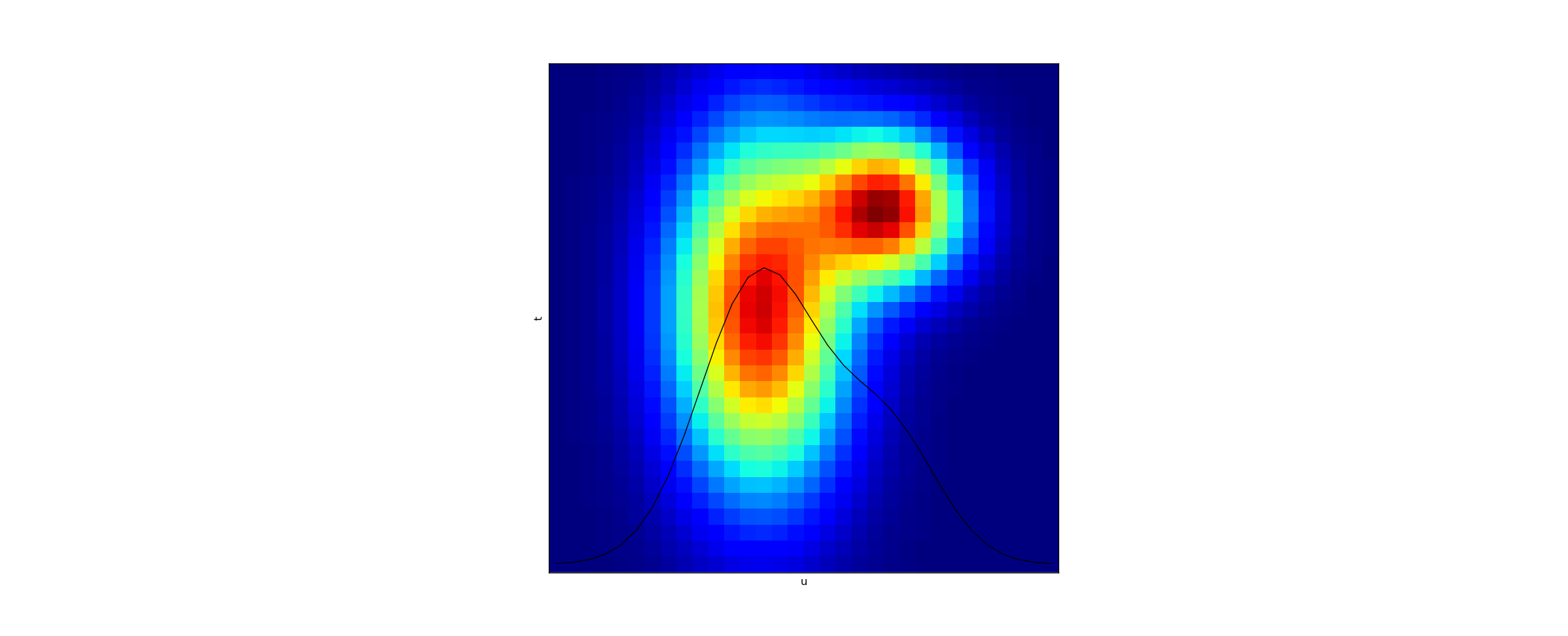
Then the result of bind is a new probability which results by taking a vertical slice, at the x-coordinate u, and summing over the vertical line. This is, of course, purely a function of u now since all the dependence on t has been averaged out. The result of summing is displayed in the graph via the black line, interpreted as a 1-dimensional plot of u.
How to do it in practice?
Lets now consider a concrete question. I have a Bernoulli event, for example visitors arriving at a webpage. I've now run an experiment and measured 53 conversions out of 200 visitors. Computing the posterior on the true conversion rate is a straightforward matter that I've discussed previously:
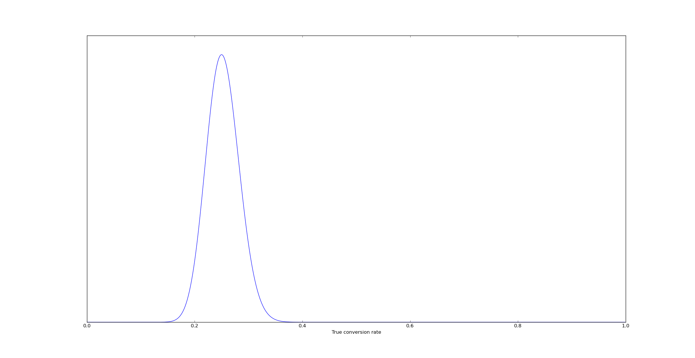
But the question arises - what empirical conversion rate can we expect over the next 100 visitors? This is now a question that's straightforwardly answered with the probability monad. We do this as follows:
val empiricalCR = for {
   l <- new Beta(51, 151)
   n <- Binomial(100, l)
   } yield (n/100.0)
(In case you are wondering, this is valid scala breeze code, just import breeze.stats.distributions._.)
The result of this is a probability distribution describing the empirical conversion rate. We can draw samples from it and plot a histogram:
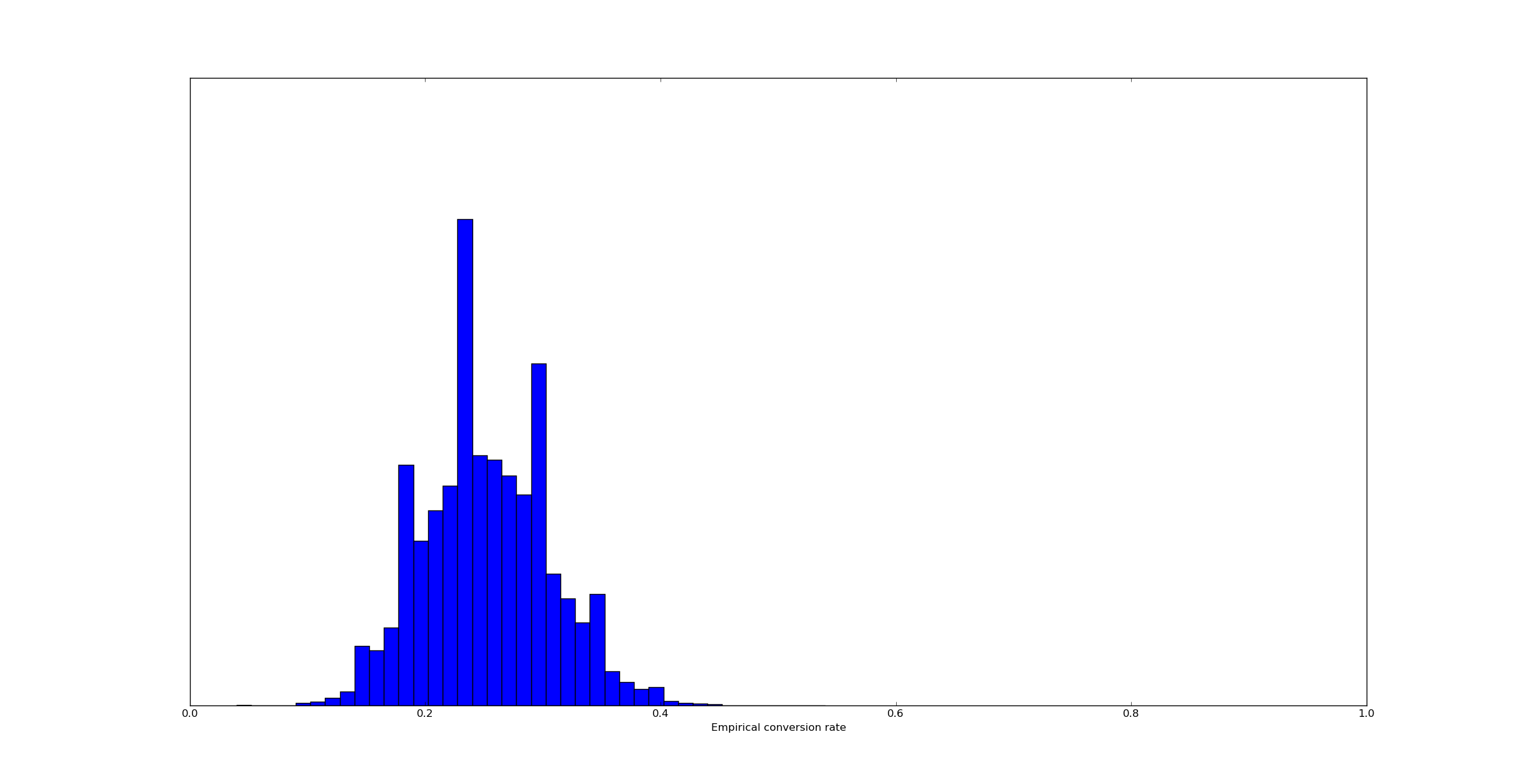
The resulting distribution is a bit wider than the distribution of the true conversion rate. That makes intuitive sense - the empirical conversion rate has two sources of variance, uncertainty in the true conversion rate and uncertainty in the binomial distribution of 100 samples.
What's happening under the hood
In the realm of pure mathematics, what's happening here is pretty simple.
When you have a probability distribution on a space T, you have a measure mu mapping (some) subsets of T into [0,1]. I.e. you have a function mu: Meas[T] => [0,1]. Hear Meas[T] represents the measurable subsets of T - for simplicity, if T were simply the integers than Meas[T] could just be all sets of integers.
A nondeterministic model would be a function f: t => Meas[U]. Then the map operation mu.map(f) would have type mu.map(f): Meas[T x U] => [0,1] - i.e., it would be a measure on the product space T x U consisting of pairs of elements (t,u).
Finally, the flatMap operation would consist of mapping, but then integrating over the T variable.
As noted earlier, this is described in much greater detail in A Categorical Approach to Probability Theory (by Giry) and A Categorical Foundation for Bayesian Probability (by Culbertson and Surtz). So this approach is both practical and also on solid theoretical footing.
Implementing it in less advanced languages
We can of course do the same calculations manually. In python, the following vectorized code seems to work in this particular case:
l = beta(51, 151).rvs(1024*1024)
n = binom(100, l).rvs()
But this would be trickier in more general cases. For example:
val funkyDistribution = for {
   l <- new Beta(51, 151)
   d <- if (l < 0.5) { Normal(5, 1) } else { Normal(-5, 1) }
} yield (d)
It's always possible, of course, to simply hack something together. Because this approach is on solid theoretical footing, one can derive results solely within the language of probability theory, and then take the result and turn it into python code.
But I personally favor the programmatic approach - it's always easier for me when the theory maps directly onto the code.
Conclusion
Probability is a monad. This allows us to take probabilistic models with deterministic inputs, and flatmap them together to build full-on probabilistic models. This can be done either mathematically (in order to derive a model to build) and much of it can be done programmatically. It's a great way to make statistical models composable, which is a very important real world consideration. Deriving probabilistic models from deterministic inputs is easy, and chaining easy steps together is usually a lot more straightforward than actually solving the full problem in one shot.